Advances in Bayesian Methods for High-Dimensional Environmental Data.

(1)

ABSTRACT

WILSON, T. ANDER. Advances in Bayesian Methods for High-Dimensional Environmental Data. (Under the direction of Brian J. Reich.)

In many applications there is prior knowledge to support a monotone relationship between

the exposure and an outcome. In these situations, statistical models can be improved by

incorpo-rating prior knowledge of a monotonic relationship. In this dissertation, we present

methodolo-gies to monotone regression in hierarchical and spatial models with applications to

environmen-tal statistics. The first case looks at hierarchical dose-response estimation in high-dimensional

toxicology experiments. The second case looks at spatially-varying bivariate exposure-response

function with monotonicity constraints in the context of multi-city air pollution studies. In

ob-servational studies, such as the air pollution example, the results can be sensitive the the choice

of confounding variables included in the model. The third part of this dissertation presents

methodology to selecting confounders in observational studies.

High-throughput screening (HTS) of environmental chemicals is used to identify chemicals

with high potential for adverse human health and environmental effects from among the

thou-sands of untested chemicals. Predicting physiologically-relevant activity with HTS data requires

estimating the response of a large number of chemicals across a battery of screening assays based

on sparse dose-response data for each chemical-assay combination. Many standard dose-response

methods are inadequate because they treat each curve separately and under-perform when there

are as few as six to ten observations per curve. We propose a semiparametric Bayesian model

for monotone dose-response estimation that borrows strength across chemicals and assays. Our

method directly parametrizes the efficacy and potency of the chemicals as well as the

proba-bility of response. We use the ToxCast data from the U.S. Environmental Protection Agency

(EPA) as motivation. We demonstrate that our hierarchical method provides more accurate

estimates of the probability of response, efficacy, and potency than separate curve estimation in

(2)

the ToxCast data to well-characterized reference chemicals on estrogen receptor α (ERα) and

peroxisome proliferator-activated receptor γ (PPARγ) assays, then estimate the probability

that other chemicals are active at lower concentrations than the reference chemicals.

Climate change is expected to alter the distribution of ambient ozone levels and temperatures

which, in turn, may impact public health. Much research has focused on the effect of short-term

ozone exposures on mortality and morbidity while controlling for temperature as a confounder,

but less is known about the joint effects of ozone and temperature. The extent of the health

effects of changing ozone levels and temperatures will depend on whether these effects are

additive or synergistic. In this dissertation we propose a spatial, semi-parametric model to

estimate the joint ozone-temperature risk surfaces in 95 US urban areas. Our methodology

restricts the ozone-temperature risk surfaces to be monotone in ozone and allows for both

non-additive and non-linear effects of ozone and temperature. We use data from the National

Mortality and Morbidity Air Pollution Study (NMMAPS) and show that the proposed model

fits the data better than additive linear and non-linear models. We then examine the synergistic

ozone-temperature effect both nationally and locally and find evidence of a non-linear ozone

effect and an ozone-temperature interaction at higher temperatures and ozone concentrations.

When estimating the effect of an exposure or treatment on an outcome, such as the effect of

ozone on mortality, it is important to select the proper subset of confounding variables to include

in the model. Including too many covariates increases mean square error on the effect of interest

while not including confounding variables biases the exposure effect estimate. We propose a

decision-theoretic approach to confounder selection and effect estimation. We first estimate the

full standard Bayesian regression model and then post-process the posterior distribution with

a loss function that penalizes models omitting important confounders. Our method can be fit

easily with existing software and in many situations without the use of Markov chain Monte

Carlo methods, resulting in computation on the order of the least squares solution. We prove

that the proposed estimator has attractive asymptotic properties. In a simulation study we

(3)

(4)

Advances in Bayesian Methods for High-Dimensional Environmental Data

by

T. Ander Wilson

A dissertation submitted to the Graduate Faculty of North Carolina State University

in partial fulfillment of the requirements for the Degree of

Doctor of Philosophy

Statistics

Raleigh, North Carolina

2014

APPROVED BY:

Montserrat Fuentes David M. Reif

Ana-Maria Staicu Brian J. Reich

(5)

DEDICATION

(6)

BIOGRAPHY

The author was born in Newton, Massachusetts. He graduated from Newton North High School

and matriculated to the University of Vermont. After graduating with a Bachelors of Arts

Degree in mathematics and taking a ten month hiatus to kayak and ski, he became a senior

programmer analyst at Mathematica Policy Research in Cambridge, Massachusetts. After four

years of nutrition and health policy research at Mathematica Policy Research, he enrolled in

the North Carolina State University Department of Statistics where he received a Masters of

(7)

ACKNOWLEDGEMENTS

I would like to thank my parents and Abby for their unending support and encouragement, and

my advisor, Dr. Brian Reich, for his guidance and patience along the way. In addition, I would

like to thank my collaborators and EPA mentors: Drs. David Reif, Ana Rappold, and Lucas

Neas.

I would also like to thank my funding sources. NIH training grant GM081057: Biostatistics

Training in the Omics Era provided funding for my first three years. This includes the funding for

material presented in Chapter 2. In addition, the research in Chapter 3 was supported in part by

an appointment to the Research Participation Program for the U.S. Environmental Protection

Agency, Office of Research and Development, administered by the Oak Ridge Institute for

Science and Education through an interagency agreement between the U.S. Department of

(8)

LIST OF TABLES

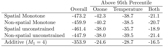
Table 3.1 Difference in cross-validation deviance from linear additive model (NMMAPS

model). . . 37

Table 3.2 Mean log RR on high and moderate temperature days over the observed and

common ozone rates by region (in percent change in mortality per 10 ppb increase in ozone). . . 43

Table 3.3 Percent increase in mortality associated with an increase from the medians

of ozone and temperature to the 95th percentiles of ozone and temperature using different models. . . 45

Table 4.1 Simulation results for design 1. Bias, MSE, and coverage (Cover) are for the

effect of interest ˆβ_x. Coverage is 95% confidence or credible interval coverage.

CPU Time is reported in seconds on a MacBook Pro with OS X, 8 GB RAM, and 2 GHz Intel Core i7. SEs for the AUC range from 0.002 to 0.004, and for CPU time from less than 0.001 to 0.498. . . 67

Table 4.2 Simulation results for design 2. Bias, MSE, and coverage (Cover) are for the

effect of interest ˆβ_x. Coverage is 95% confidence or credible interval coverage.

CPU Time is reported in seconds on a MacBook Pro with OS X, 8 GB RAM, and 2 GHz Intel Core i7. SEs for the AUC range from less than 0.001 to 0.006,

and for CPU time from less than 0.001 to 0.003. . . 68

Table A.1 Simulation results for mean response and probability of active response. The displayed values are the mean (standard error) across simulated data sets. RMSE is the pointwise root mean square error taken over 50 evenly spaced points on log base 3, the spacing scale for concentrations in the real data. RMSE Top and RMSE AC50 are only calculated for dose-response curves that are active. AUC is the area under the ROC curve. . . 92

(12)

LIST OF FIGURES

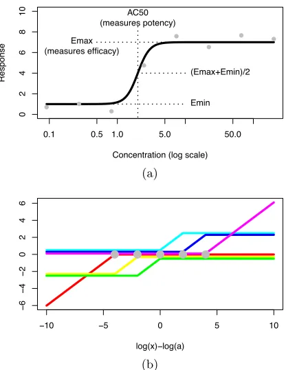
Figure 2.1 Panel (a) shows an annotated example of the four-parameter log-logistic

(FPLL) function. The FPLL model is f(x;t, b, a, w) = t−(t −b)×Logit

[−w{log(x)−log(a)}], where x is the tested concentration and (t, b, w, a)

parameterizes the Emax, Emin, AC50, andw(rate of increase), respectively.

Panel (b) shows six sample basis functions with internal knots (−4,−2,0,2,4)

marked with gray circles. This figure appears in color in the electronic version

of this article. . . 8

Figure 2.2 Illustration of the ToxCast data structure showing 20 chemicals tested on 8

assays. This is a sample of the 309 chemicals and 81 assays used in Section 2.5 with curves as reported in the publicly available ToxCast data. All 309

chemicals are tested on all 81 assays, resulting in 309×81 = 25,029

chemical-assay combinations. This figure appears in color in the electronic version of this article. . . 11

Figure 2.3 Example of ZIPLL and ToxCast estimates for 12 chemicals on the PXRE

assay. The ZIPLL posterior mean (thick solid black line) with 95% poste-rior intervals (dashed black lines), and the ToxCast fit (thin solid gray line) are shown. The legend shows a binary indicator of an active response from ToxCast (1=active) and the posterior probability of an active response us-ing ZIPLL. The FPLL fits are redrawn from the parameter estimated in the ToxCast public release data. This figure appears in color in the electronic version of this article. . . 18

Figure 2.4 Panel (a) plots the number of assays each chemical responded on with 95%

posterior intervals. The simultaneous fitting of all chemical-assay combina-tions allows for the estimation of the joint distribution of assays and naturally

propagates the distribution of the total number of assay responses. Thex

in-dicates the number of assay responses reported in the ToxCast data. (The 309 chemical names are omitted on the horizontal axis for readability.) Panel (b) shows posterior mean random intercept for the assay probability of

re-sponse (δj) as discussed in Section 2.3.2 and 95% posterior intervals. This

figure appears in color in the electronic version of this article. . . 20

Figure 2.5 Chemical ranks by potency with 90% credible intervals. The x-axis shows

the posterior mean AC50 (more potent to the left). The y-axis ranks the chemicals by potency (most potent, rank one, at top). All chemicals with at

least a 0.50 percent probability of active response are plotted. For PPARγand

ERα reference chemicals are marked for comparison. These chemicals have

shown documented activity on these assays. This figure appears in color in the electronic version of this article. . . 22

Figure 2.6 Posterior probability that chemicals are more active than selected reference

chemicals on PPARγ. All chemicals with at least a 0.05 probability of being more active than all three reference chemicals are shown and ordered by their

(13)

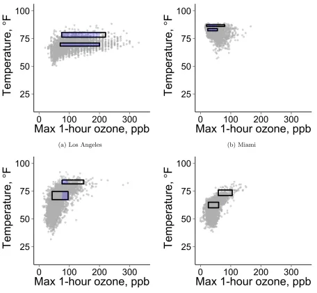
Figure 3.1 Ozone-temperature distribution for selected cities. The upper and lower boxes contain data for high temperature days and moderate temperature days, re-spectively, over the observed ozone range. The purple subsections highlight the common ozone range, the intersection of the ozone ranges for high and moderate temperature days. Details on the definition used to identify these days are in Section 3.3.3. Seattle is the only city in the dataset that does not have a common ozone range. . . 27

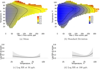
Figure 3.2 Panels (a) and (b) show the pointwise mean and standard deviation of the

national log RR surfaces. Panels (c) and (d) show cross section of the log RR surface with ozone fixed at 50 and 100 ppb, respectively, along with 95% posterior intervals. Log RR is in percent change in mortality per one ppb increase in ozone. . . 38

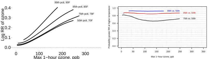
Figure 3.3 Comparison of the log RR at the 50th, 75th, 95th, and 99th percentiles of

temperature. The estimates extend over the range of ozone values observed in at least 5 cities. Subfigure 3.3a shows the mean log RR for each cross-section and Subfigure 3.3b shows the pointwise posterior probability that log RR is greater at the high temperature. Log RR is in percent change in mortality

per one ppb increase in ozone. . . 40

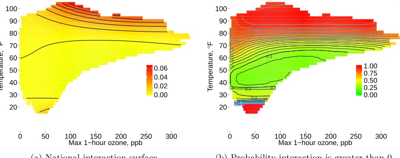
Figure 3.4 National interaction surface and pointwise probability of positive interaction.

Panel 3.4a shows the national interaction surface which is the cross-derivative of the log risk surface or the derivative of the log RR surface with respect to temperature. This shows how log RR changes with temperature and quanti-fies the interaction at each point. Panel 3.4b show the probability that the national interaction surface is greater than 0. . . 41

Figure 3.5 Log RR surfaces for selected cities (left) and their pointwise standard

devia-tions (right). Surfaces are plotted only over the range of data observed data for that city. The cities were selected for being geographically diverse and having varied ozone and temperature ranges. . . 42

Figure 3.6 Comparison of the log RR at high temperature and moderate temperatures

as defined in Section 3.3.3. Panel 3.6a compares the ratio of log RR over the observed ozone range (black) and common ozone range (blue). The posterior mean and 95% interval are shown. Panel 3.6b shows a map of the ratio on days in the common ozone range. Cities outlined in black (Los Angeles and St. Louis) are significant at the 0.8 level. . . 44

Figure 4.1 Probability of including covariates for simulation design one withn= 100 for

the credible region method ( ), BAC (_#), BMA (4) , and adaptive LASSO

(+). Left: the proportion of simulated data sets for which each variable is selected. For BMA and BAC a variable is counted as included if its inclusion probability is greater than 0.5. Right: the average inclusion probability for BMA and BAC. Covariates in the first section (1 to 7) are confounders, in the second section (8 to 14) are other explanatory variables, and the far right

(14)

Figure 4.2 AUC for simulation design one withp > nfor three different rates of growth

forn. . . 60

Figure 4.3 Solution path for three subgroups and overall. The thick black line is the

estimated PM effect, βˆ_x. The other lines are the estimates for the other

covariates in the model. The regression coefficients correspond to centered

and scaled variables. . . 64

Figure 4.4 Estimates of the PM effect ( ˆβ_x). Top: The point estimates with each model

and the 95% interval. Bottom: The ratio of the SE or SD of ˆβ_x with each

model compared to the full OLS model. . . 65

Figure A.1 Example of simulated regression functions under using ZILL A.1a and

mix-ture of normals A.1b. . . 90

Figure A.2 Comparison of the posterior probability of an active response estimated with ZIPLL (x-axis) and the binary indicator of active response from ToxCast (y-axis) for all 309 chemicals on three assays. The majority of chemicals are considered not active (clustered in bottom left) or active (upper right) with both methods. However, using ZIPLL we estimated that several chemicals have posterior probabilities of response between 0.1 and 0.9, suggesting that there is not conclusive evidence that these chemical responded or not, but are forced to be classified as either active or not in the ToxCast data. . . 93

Figure B.1 Summary of the ozone and temperature distribution. . . 95 Figure B.2 Demonstration of the different basis expansions used in the first and second

stages. The bottom left shows the observed ozone-temperature distribution in each city. To the right are the basis functions in the temperature direction and to the top are the basis functions in the ozone direction for each stage. The first stage basis functions are different in each city. . . 96 Figure B.3 Difference in deviance from the linear, additive model (NMMAPS model) for

the spatial monotone model with different numbers of basis functions in the

ozone (M1) and temperature (M2) directions. . . 97

Figure B.4 Average rank of CV results across Figures B.3a through B.3d, with one being

the best performing model. The best model on average was (M1, M2) = (7,9)

with an average rank of 3.75; this is the model used for analysis. The next best models were (9,10), (10,9), and (9,9) with average ranks of 5.25, 5.50, and 6.75, respectively. . . 98 Figure B.5 Trace plots of the point wise estimates of the risk surface. . . 102

Figure B.6 Trace of the posterior sample of logρ(log range in log kilometers). The trace

plot only includes the posterior sample and does not show the portion of the burn in portion of the chain. The posterior mean is 922.9, the median is

(15)

Figure C.1 Comparison of model selection methods for simulation design 1. Subfig-ure C.1a shows the AUC while the remaining subfigSubfig-ures compare model size and performance with different selection criteria. The criteria are forward

selection with αf s = 0.25 (solid; ——), forward selection with αf s = 0.15

(short dash gray; - - - -), Cp (dotted; · · · ·), CV (short dash blue;

--), AIC (dash-dot-dash; -·-·-·-), and BIC (long dash; — — — —). Model

size is the number of confounders selected and does not count the outcome

(16)

Chapter 1

Introduction

1.1

Introduction

In many applications there is scientific evidence that an exposure’s effect on an outcome may

be monotonic in nature. In such situations, statistical estimation of the exposuresponse

re-lationship can be improved by incorporating prior knowledge of monotonicity into the model.

Many methods have been developed for monotonic regression (e.g. Friedman and Tibshirani,

1984; Mukerjee, 1988; Mammen, 1991; Hall and Huang, 2001; Holmes and Heard, 2003; Neelon

and Dunson, 2004; Wang and Leng, 2008; Curtis and Ghosh, 2011a). In this dissertation, we

develop methodology for monotonic regression in hierarchical and spatial models with

applica-tions to environmental exposures. In the first chapter, we use a hierarchical Bayesian model to

estimate dose-response relationships in the context of high-dimensional toxicology studies. In

this setting, the designed toxicology experiment results in data with a known non-decreasing

relationship between dose and multiple in vitro outcomes. In the second chapter, we use a

spatial model to estimate bivarite, semi-paraemtric risk surfaces in different locations. In this

case, we are interested in the effect of co-exposures to ozone and temperature on mortality

and assume that the ozone effect has a monotonic relationship with mortality. In observational

(17)

can be sensitive to the choice of confounding variables included in the model. In Chapter 4 we

present methodology to choose confounding variables in observational studies.

1.1.1 Hierarchical Monotone Dose-Response Modeling for High-Throughput Toxicity Screening of Environmental Chemicals

There are thousands of untested chemicals in common use today (Judson et al., 2009).

Com-prehensive testing of all chemicals is not feasible due to the financial and temporal costs of

traditional chemical testing, which relies heavily on animal testing. Recently, efforts have been

made to prioritize the large number of untested chemicals so that available testing resources can

be targeted at those chemicals that are most likely to cause adverse health or environmental

effects. This approach combines high-thoughput screening (HTS) which tests chemicals on a

large battery of relatively fast and inexpensive bioassays and predictive models.

The data for each chemical-assay combination consists of dose-response pairs and are often

known to have a monotonic relationship. Large designed experiments such as the US

Environ-mental Protection Agency’s (EPA) ToxCast which tests thousands of chemicals on hundreds

of HTS assays can result in large datasets (Dix et al., 2007; Kavlock et al., 2012). However,

the data for each chemical-assay combination can be sparse. Hence, HTS data consists of a

large number of sparse dose-response relationships from which we seek to rank chemicals based

on their relative bioactivity as measured on HTS assays as well as estimate key parameters

used in existing predictive model. As such, statistical methods are needed that estimate the

dose-response relationship in a way that parameterizes key statistics and facilitates ranking

of chemicals and other between chemical comparisons. At the same time, these methods must

be robust to the sparsity of data observed in each chemical-assay combination, presumably by

sharing information across the large number of chemical-assay pairs, and being efficient enough

to allow for estimation of large HTS datasets.

In Chapter 2 we present a hierarchical Bayesian model for the estimation of monotone

(18)

summary statistics used in predictive models – the potency, efficacy, and probability of an active

response – while allowing for flexibility of the shape of the dose-response relationship. Using

the proposed method, we estimate the dose-response relationship of a subset of the ToxCast

data and rank chemicals based on their potential potency on key bioassay.

1.1.2 Modeling the Effect of Temperature on Ozone-Related Mortality

The EPA has concluded that current scientific evidence supports a causal relationship between

ozone and respiratory health effects and a likely to be causal relationship between ozone and

cardiovascular health effects and mortality (US EPA, 2013). Several observational studies have

associated ambient ozone exposures with increased rates of mortality while controlling for

tem-perature and other confounding variables (Bell et al., 2004), while clinical research has found

that ozone’s effect on lung function is monotonicly increasing (McDonnell et al., 2012). With

the onset of anticipated climate changes (National Research Council, 2004a) both ozone and

temperature distributions are expected to increase in the near future (US EPA, 2009). To

antic-ipate the health burden of these changes it is important to understand the joint health effects

of ozone and temperature.

Many multi-city time-series studies have associated ambient ozone exposures with increased

risk of non-accidental mortality while controlling for temperature (Bell et al., 2004, 2006; Smith

et al., 2009). These results includes evidence of a non-linear ozone effect (Bell et al., 2006) and a

potentially greater linear ozone effect at higher temperatures than at lower temperatures (Smith

et al., 2009). However, estimates of interaction based on comparing the linear ozone effect at

different temperatures may be confounded by the different ozone distributions observed at

different temperatures and non-linearity in the ozone effect. To isolate interaction it is essential

to compare the ozone effect at different temperatures but for the same ozone level.

One way to isolate interaction is to estimate the full ozone-temperature risk surface. By

estimating the bivariate risk surface the rate of change in risk associated with changes in ozone

(19)

Hence, comparisons of the ozone effect can be made at different temperatures but for the same

ozone level. This approach has recently been employed in the single-city setting (Ren et al.,

2008; Chen et al., 2013) and visual inspection of the estimated risk surfaces suggests that there

is a non-linear and non-additive joint ozone-temperature effect.

There are several challenges to estimating ozone-temperature risk surfaces in multi-city

studies. Chief among them is the substantially different ozone and temperature ranges observed

in each city. As a result, it is challenging to find a parameterization of the risk surface that is

appropriate to use at all locations, while using a different basis expansion at each city does not

allow for the use of existing estimation methods such as those used in Dominici et al. (2002). In

addition, there is a computational burden associated with estimating surface models at many

locations. These issues are addressed in Chapter 3 which details a model for spatially-varying

risk surfaces which are constrained to be monotone in ozone.

1.1.3 Confounder Selection via Penalized Credible Regions

In many observations studies the primary interest lies in estimating the effect of an exposure

on an outcome while controlling for a large number of potential confounding variables. In such

cases, the exposure effect can be sensitive to the choice of confounding variables included in

the model. The sensitivity to confounder selection in multi-city time-series studies, such as the

work presented in Chapter 3, has been documented by Sacks et al. (2012). Omitting important

confounding variables, those correlated with both the outcome and the exposure, can bias the

exposure estimate while including too many covariates independent of both the outcome and

exposure can inflate the variance of the effect estimate. In problems where the primary interest

is in parameter estimation it is important to select an appropriate subset of the potentially

large number of confounding variables.

There are ample variable selection methods available. These include: all subsets, forward

selection, an array of penalized regression methods (Tibshirani, 1996; Fan and Li, 2001; Zou

(20)

McCulloch, 1993; George and Foster, 2000; Brown et al., 2002; Carvalho et al., 2010; Bondell and

Reich, 2012), among others. Variable selection, in general, focuses on balancing parsimony and

model fit as estimated by minimizing the sum of squared errors. These methods can be highly

effective in selecting variables for prediction, but can be biased for effect estimation. Bayesian

model averaging (BMA) attempts to average the effect estimates over the model space giving

more weight to models that have greater support from the data. However, BMA also tunes

for prediction and can result in biased estimates of the effect of interest when the exposure

is correlated with other covariates. Hence, a new class of selection methods are needed that

explicitly treat one covariate as the exposure or treatment of interest and focus on estimating

the associated regression coefficient.

To address the issue of confounder selection and effect estimation Crainiceanu et al. (2008)

proposed a two-stage approach. In the first stage, the exposure of interest is regressed on the

covariates to identify potential confounders that are correlated with the exposure of interest.

Then, in the second stage, the outcome is regressed on the exposures of interest and the other

observed covariates to identify additional covariates correlated with the outcome that were

not identified as potential confounders in the first stage. Bayesian adjustment for confounding

(BAC; Wang et al., 2012) formalized these two steps into a Bayesian approach that estimates

the two models simultaneously with a model-averaging approach. BAC proved effective at large

sample sizes; however, it was biased at small sample sizes, lacked optimality properties and is

computationally inefficient.

Chapter 4 of this thesis presents a new method for confounder selection. The proposed

method takes a decision-theoretic approach following that of Bondell and Reich (2012) but uses

an exposure model and a loss function that explicitly penalizes models that omit important

confounding variables. Chapter 4 details the methodology and presents simulation studies and

(21)

Chapter 2

Hierarchical Dose-Response

Modeling for High-Throughput

Toxicity Screening of Environmental

Chemicals

2.1

Introduction

There are thousands of untested chemicals in common use. Comprehensive toxicity testing of

all chemicals is infeasible due to high monetary and temporal costs (Judson et al., 2009). To

address this problem, a new paradigm in toxicity testing focuses on screening larger numbers

of chemicals on a diverse battery of relatively quick and inexpensive high-throughput screening

(HTS) assays that measure a variety of cellular and biochemical responses. Each assay measures

a single endpoint, such as transcription of a target gene or binding to a specific receptor protein.

The aim of HTS is to predict which chemicals are most likely to perturb normal biological

processes that lead to adverse human health and environmental effects, and focus scarce testing

(22)

To predict potential chemical activity from HTS data requires statistical models to estimate

the response of each chemical on each assay and to compare and rank chemicals. There are

three main quantities used to compare chemicals: 1) the probability that an active response

occurred, 2) the potency or concentration at which a response occurs, and 3) the efficacy or

magnitude of the response. These three quantities form the basis of chemical prioritization.

With improved estimates of these three quantities, predictive models will be able to better

predict which chemicals are most likely to have potentially hazardous effects.

Dose-response modeling for HTS data is unique because there are a large number of curves

to estimate but the data for each curve are sparse. For example, the ToxCast project at the US

EPA (Dix et al., 2007; Kavlock et al., 2012) has screened nearly 2,000 chemicals on over 700 HTS

assays; however, each chemical-assay combination is tested at six to ten unique concentrations

and, in most cases, in singlicate at each concentration. Analysis is further complicated by

assay and chemical effects, such as assays that are more or less sensitive, correlated assays

that measure the same or similar cellular response, and chemicals that are highly active or not

active on a variety of assays. Hence, HTS requires a dose-response method that is robust to the

sparsity of the data for each chemical-assay combination, takes advantage of the larger number

of chemicals and assays, and accurately estimates the efficacy, potency, and probability of an

active response.

A variety of parametric models are used for estimating monotonic dose-response curves

(Ritz, 2010). The most common method is the four-parameter log-logistic model (FPLL) which

directly parameterizes the efficacy and potency with the Emax (maximal response or upper

asymptote) and AC50 (concentration at which the half maximal response occurs), respectively.

Figure 2.1a shows an annotated example FPLL dose-response curve. The current release of EPA

ToxCast results uses FPLL to fit each dose-response curve with least squares (Judson et al.,

2010). Fitting six to ten observations with a four-parameter model using least squares results in

poor variance estimates (currently not provided in the ToxCast public release) and no estimates

(23)

0.1 0.5 1.0 5.0 50.0

0

2

4

6

8

10

Concentration (log scale)

Response

Emax (measures efficacy)

Emin AC50

(measures potency)

(Emax+Emin)/2

● ● ●

● ●

●

(a)

−10 −5 0 5 10

−

6

−

4

−

2

0

2

4

6

log(x)−log(a)

● ● ● ● ●

(b)

Figure 2.1: Panel (a) shows an annotated example of the four-parameter log-logistic (FPLL)

function. The FPLL model is f(x;t, b, a, w) =t−(t−b)×Logit [−w{log(x)−log(a)}], where

x is the tested concentration and (t, b, w, a) parameterizes the Emax, Emin, AC50, and w

(rate of increase), respectively. Panel (b) shows six sample basis functions with internal knots

(−4,−2,0,2,4) marked with gray circles. This figure appears in color in the electronic version

of this article.

There are several available frequentist approaches for monotonic curve estimation (e.g.

Fried-man and Tibshirani, 1984; Mukerjee, 1988; Mammen, 1991; Hall and Huang, 2001; Mammen

et al., 2001; Wang and Li, 2008). Recently, several semiparametric Bayesian methods for

mono-tone regression for a single curve have been proposed. Holmes and Heard (2003) proposed using

piecewise constant functions with random knots, Neelon and Dunson (2004) utilized a piecewise

linear spline model, and Curtis and Ghosh (2011a) developed a Bernstein polynomial model.

Also, Shively et al. (2009) modeled the monotonic function as the integral of a positive function.

None of these general semiparametric regression methods directly parameterize the efficacy or

(24)

predictive modeling.

Our problem is different from these because we are estimating the response for several

chemicals on multiple assays. Bayesian hierarchical models have been used in many fields where

the data takes a natural hierarchical structure. Severalin vivoor developmental toxicity studies

have used Bayesian hierarchical models to improve estimates when measuring the response of

multiple correlated endpoints tested with a single chemical (e.g Faes et al., 2006; Choi et al.,

2010) or used a multivaraite model that assumes correlation in residuals for multiple health

outcomes (Neelon and Dunson, 2004).

To incorporate dependence in the regression function between four HTS assays and eight

nanomaterials, Patel et al. (2012) estimate dose-duration-response surfaces using linear

B-splines with two internal knots in both the duration and dose direction. The first knot

param-eterizes potency with the no observable adverse effect level (NOAEL), an alternative measure

to AC50. For each chemical, they model correlation in the knot location and basis coefficients

across the assays, but they do not model correlation across chemicals within assay. While the

direct parameterization of the NOAEL is appealing, this model does not directly parameterize

the probability of a response or the efficacy, two important parameters for prioritization. In

addition, the model does not include assay effects which we assume to exist in our data and

can potentially improve fitting with the large number of chemicals but small sample size with

each chemical-assay. While the simple choice of linear splines with two internal knots provides

for a reasonable size model for a generalized additive model, this basis is not realistic for a

one-dimensional model (dose only, not dose-duration surfaces).

In this paper, we propose a Bayesian hierarchical model for dose-response curves that is

specifically tailored to the high-dimensional, sparse data setting of the ToxCast project, called

the zero-inflated piecewise log-logistic model (ZIPLL). ZIPLL is a mixture between a non-active

response and an active response that extends FPLL to a more flexible spline formulation while

maintaining direct parameterization of the efficacy and potency of each chemical-assay

(25)

of uncertainty for ranks of efficiency and potency which should allow for decision-makers to use

the results appropriately when deciding which chemicals to consider for future, more

compre-hensive, testing. We use a hierarchical framework that borrows strength across chemicals and

assays. This adds robustness, incorporates assay and chemical effects, and allows for estimation

of joint distributions of responses across multiple assays. In addition, prior information and

covariates can be included to exploit known relationships between chemicals, between assays,

and between chemical-assay combinations.

2.2

The ToxCast Data

The ToxCast project uses a diverse battery of HTS assays and informatic models to rapidly

characterize the activity of thousands of chemicals. These chemical activity profiles are used to

support decisions regarding prioritization for further testing (Reif et al., 2010), predictin vivo

activity (Martin et al., 2011), and inform risk assessments (Judson et al., 2011). In support

of these goals, the ToxCast project has tested over 2,000 chemicals on over 700 HTS assay

endpoints for which analysis is ongoing. The data for the first 309 chemicals tested for Phase I

are publicly available (http://www.epa.gov/ncct/toxcast/data.html). Figure 2.2 illustrates the

unique structure of the data.

In this paper we use the 309 chemicals in the publicly available data and a subset of 81

as-says comprising the multiplexed transcription factor reporter platform (Romanov et al., 2008,

www.attagene.com). This platform enables high-content, functional assessment of

transcrip-tion factor activity, which is a core component of cellular gene regulatory networks. Both

cis-regulating response element constructs (CIS) and trans-activating (TRANS) potential of

multiple nuclear hormone receptors are measured. These 48 CIS and 25 TRANS assays (plus

8 negative control assays) address relevant cellular processes including response to xenobiotics,

genotoxic stress, hypoxia, oxidative damage, immune-modulation, and endocrine disruption.

Martin et al. (2010) evaluated these assays’ response to the 309 Phase I chemicals.

(26)

Index Index Cyprodinil Index Diazinon Index Dichlor an Index Iprodione Index Isaz ofos Index Isoxaben Index Lactof en Index Lindane Index Linuron Index Rotenone Index Setho xydim Index Index Vincloz olin Zoxamide Index "n" Ahr_CIS ● ● ● ● ● ● ●

c(as.matrix(webdat[which(webdat$chemical_casrn == chemid), conccols]))

c(as

.matr

ix(w

ebdat[which(w

ebdat$chemical_casr

n == chemid), respcols]))

● ● ● ● ● ● ●

c(as

.matr

ix(w

ebdat[which(w

ebdat$chemical_casr

● ● ● ● ● ●●

c(as

.matr

ix(w

ebdat[which(w

ebdat$chemical_casr

● ● ● ●● ● ●

c(as

.matr

ix(w

ebdat[which(w

ebdat$chemical_casr

● ● ● ● ● ●●

c(as

.matr

ix(w

ebdat[which(w

ebdat$chemical_casr

● ● ● ● ●● ●

c(as

.matr

ix(w

ebdat[which(w

ebdat$chemical_casr

● ● ● ● ●● ●

c(as

.matr

ix(w

ebdat[which(w

ebdat$chemical_casr

● ● ● ● ● ● ●

c(as

.matr

ix(w

ebdat[which(w

ebdat$chemical_casr

● ● ● ● ● ●●

c(as

.matr

ix(w

ebdat[which(w

ebdat$chemical_casr

● ● ● ● ● ● ●

c(as

.matr

ix(w

ebdat[which(w

ebdat$chemical_casr

● ● ● ● ● ● ●

c(as

.matr

ix(w

ebdat[which(w

ebdat$chemical_casr

● ● ●

c(2, 2, 2)

c(0.5, 2, 3.5)

● ● ● ● ● ● ●

c(as

.matr

ix(w

ebdat[which(w

ebdat$chemical_casr

● ● ● ● ● ● ● c(as .matr ix(w ebdat[which(w ebdat$chemical_casr

Index

"n"

AP_1_CIS

● ● ● ● ● ●●

c(as

.matr

ix(w

ebdat[which(w

ebdat$chemical_casr

● ● ● ● ● ● ●

c(as

.matr

ix(w

ebdat[which(w

ebdat$chemical_casr

● ● ● ● ● ● ●

c(as

.matr

ix(w

ebdat[which(w

ebdat$chemical_casr

● ● ● ● ● ● ●

c(as

.matr

ix(w

ebdat[which(w

ebdat$chemical_casr

● ● ● ● ● ● ●

c(as

.matr

ix(w

ebdat[which(w

ebdat$chemical_casr

● ● ● ● ● ● ●

c(as

.matr

ix(w

ebdat[which(w

ebdat$chemical_casr

● ● ● ● ● ● ●

c(as

.matr

ix(w

ebdat[which(w

ebdat$chemical_casr

● ● ● ● ● ● ●

c(as

.matr

ix(w

ebdat[which(w

ebdat$chemical_casr

● ● ● ● ● ● ●

c(as

.matr

ix(w

ebdat[which(w

ebdat$chemical_casr

● ● ●● ●●●

c(as

.matr

ix(w

ebdat[which(w

ebdat$chemical_casr

● ● ● ● ● ● ●

c(as

.matr

ix(w

ebdat[which(w

ebdat$chemical_casr

● ● ●

c(2, 2, 2)

c(0.5, 2, 3.5)

● ● ● ● ● ● ●

c(as

.matr

ix(w

ebdat[which(w

ebdat$chemical_casr

Index

"n"

AP_2_CIS

● ● ● ● ● ● ●

c(as

.matr

ix(w

ebdat[which(w

ebdat$chemical_casr

● ● ● ● ● ● ●

c(as

.matr

ix(w

ebdat[which(w

ebdat$chemical_casr

● ● ● ● ● ● ●

c(as

.matr

ix(w

ebdat[which(w

ebdat$chemical_casr

● ● ● ● ● ● ●

c(as

.matr

ix(w

ebdat[which(w

ebdat$chemical_casr

● ● ● ● ● ● ●

c(as

.matr

ix(w

ebdat[which(w

ebdat$chemical_casr

● ● ● ● ● ● ●

c(as

.matr

ix(w

ebdat[which(w

ebdat$chemical_casr

● ● ● ● ● ● ●

c(as

.matr

ix(w

ebdat[which(w

ebdat$chemical_casr

● ● ● ● ● ● ●

c(as

.matr

ix(w

ebdat[which(w

ebdat$chemical_casr

● ● ● ● ● ● ●

c(as

.matr

ix(w

ebdat[which(w

ebdat$chemical_casr

● ● ● ● ● ● ●

c(as

.matr

ix(w

ebdat[which(w

ebdat$chemical_casr

● ● ● ● ● ● ●

c(as

.matr

ix(w

ebdat[which(w

ebdat$chemical_casr

● ● ●

c(2, 2, 2)

c(0.5, 2, 3.5)

● ● ● ● ● ● ●

c(as

.matr

ix(w

ebdat[which(w

ebdat$chemical_casr

Index

"n"

AR_TRANS

● ● ● ● ● ● ●

c(as

.matr

ix(w

ebdat[which(w

ebdat$chemical_casr

● ● ● ● ● ● ●

c(as

.matr

ix(w

ebdat[which(w

ebdat$chemical_casr

● ● ● ● ● ● ●

c(as

.matr

ix(w

ebdat[which(w

ebdat$chemical_casr

● ● ● ● ● ● ●

c(as

.matr

ix(w

ebdat[which(w

ebdat$chemical_casr

● ● ● ● ● ● ●

c(as

.matr

ix(w

ebdat[which(w

ebdat$chemical_casr

● ● ● ● ● ● ●

c(as

.matr

ix(w

ebdat[which(w

ebdat$chemical_casr

● ● ● ● ● ● ●

c(as

.matr

ix(w

ebdat[which(w

ebdat$chemical_casr

● ● ● ● ● ● ●

c(as

.matr

ix(w

ebdat[which(w

ebdat$chemical_casr

● ● ● ● ● ● ●

c(as

.matr

ix(w

ebdat[which(w

ebdat$chemical_casr

● ● ● ● ● ● ●

c(as

.matr

ix(w

ebdat[which(w

ebdat$chemical_casr

● ● ● ● ● ● ●

c(as

.matr

ix(w

ebdat[which(w

ebdat$chemical_casr

● ● ●

c(2, 2, 2)

c(0.5, 2, 3.5)

● ● ● ● ● ● ●

c(as

.matr

ix(w

ebdat[which(w

ebdat$chemical_casr

Index

"n"

BRE_CIS

● ● ● ● ●● ●

c(as

.matr

ix(w

ebdat[which(w

ebdat$chemical_casr

● ● ● ● ● ● ●

c(as

.matr

ix(w

ebdat[which(w

ebdat$chemical_casr

● ● ● ● ●● ●

c(as

.matr

ix(w

ebdat[which(w

ebdat$chemical_casr

● ● ● ● ● ● ●

c(as

.matr

ix(w

ebdat[which(w

ebdat$chemical_casr

● ● ● ● ● ● ●

c(as

.matr

ix(w

ebdat[which(w

ebdat$chemical_casr

● ● ● ● ● ●●

c(as

.matr

ix(w

ebdat[which(w

ebdat$chemical_casr

● ● ● ● ● ●●

c(as

.matr

ix(w

ebdat[which(w

ebdat$chemical_casr

● ● ● ● ● ●●

c(as

.matr

ix(w

ebdat[which(w

ebdat$chemical_casr

● ● ● ● ● ●●

c(as

.matr

ix(w

ebdat[which(w

ebdat$chemical_casr

●● ●

● ● ● ●

c(as

.matr

ix(w

ebdat[which(w

ebdat$chemical_casr

● ● ● ● ● ● ●

c(as

.matr

ix(w

ebdat[which(w

ebdat$chemical_casr

● ● ●

c(2, 2, 2)

c(0.5, 2, 3.5)

● ● ● ● ● ● ●

c(as

.matr

ix(w

ebdat[which(w

ebdat$chemical_casr

Index

"n"

CMV_CIS

● ● ● ● ●●●

c(as

.matr

ix(w

ebdat[which(w

ebdat$chemical_casr

● ● ● ● ● ● ●

c(as

.matr

ix(w

ebdat[which(w

ebdat$chemical_casr

● ● ● ● ● ● ●

c(as

.matr

ix(w

ebdat[which(w

ebdat$chemical_casr

● ● ● ● ● ● ●

c(as

.matr

ix(w

ebdat[which(w

ebdat$chemical_casr

● ● ● ● ● ● ●

c(as

.matr

ix(w

ebdat[which(w

ebdat$chemical_casr

● ● ● ● ● ● ●

c(as

.matr

ix(w

ebdat[which(w

ebdat$chemical_casr

● ● ● ● ● ● ●

c(as

.matr

ix(w

ebdat[which(w

ebdat$chemical_casr

● ● ● ● ● ● ●

c(as

.matr

ix(w

ebdat[which(w

ebdat$chemical_casr

● ● ● ● ●● ●

c(as

.matr

ix(w

ebdat[which(w

ebdat$chemical_casr

● ● ● ● ● ● ●

c(as

.matr

ix(w

ebdat[which(w

ebdat$chemical_casr

● ● ● ● ● ● ●

c(as

.matr

ix(w

ebdat[which(w

ebdat$chemical_casr

● ● ●

c(2, 2, 2)

c(0.5, 2, 3.5)

● ● ● ● ● ● ●

c(as

.matr

ix(w

ebdat[which(w

ebdat$chemical_casr

Index

"n"

CRE_CIS

● ● ● ● ● ●●

c(as

.matr

ix(w

ebdat[which(w

ebdat$chemical_casr

● ● ● ● ● ● ●

c(as

.matr

ix(w

ebdat[which(w

ebdat$chemical_casr

● ● ● ● ● ●●

c(as

.matr

ix(w

ebdat[which(w

ebdat$chemical_casr

● ● ● ● ● ● ●

c(as

.matr

ix(w

ebdat[which(w

ebdat$chemical_casr

● ● ● ● ● ● ●

c(as

.matr

ix(w

ebdat[which(w

ebdat$chemical_casr

● ● ● ● ● ● ●

c(as

.matr

ix(w

ebdat[which(w

ebdat$chemical_casr

● ● ● ● ● ● ●

c(as

.matr

ix(w

ebdat[which(w

ebdat$chemical_casr

● ● ● ● ● ● ●

c(as

.matr

ix(w

ebdat[which(w

ebdat$chemical_casr

● ● ● ● ● ● ●

c(as

.matr

ix(w

ebdat[which(w

ebdat$chemical_casr

● ● ●● ● ● ●

c(as

.matr

ix(w

ebdat[which(w

ebdat$chemical_casr

● ● ● ● ● ● ●

c(as

.matr

ix(w

ebdat[which(w

ebdat$chemical_casr

● ● ●

c(2, 2, 2)

c(0.5, 2, 3.5)

● ● ● ● ● ● ●

c(as

.matr

ix(w

ebdat[which(w

ebdat$chemical_casr

Index

"n"

DR5_CIS

● ● ● ● ● ● ●

c(as

.matr

ix(w

ebdat[which(w

ebdat$chemical_casr

● ● ● ● ● ● ●

c(as

.matr

ix(w

ebdat[which(w

ebdat$chemical_casr

● ● ● ● ● ● ●

c(as

.matr

ix(w

ebdat[which(w

ebdat$chemical_casr

● ● ● ● ● ● ●

c(as

.matr

ix(w

ebdat[which(w

ebdat$chemical_casr

● ● ● ● ● ● ●

c(as

.matr

ix(w

ebdat[which(w

ebdat$chemical_casr

● ● ● ● ● ● ●

c(as

.matr

ix(w

ebdat[which(w

ebdat$chemical_casr

● ● ● ● ● ● ●

c(as

.matr

ix(w

ebdat[which(w

ebdat$chemical_casr

● ● ● ● ●● ●

c(as

.matr

ix(w

ebdat[which(w

ebdat$chemical_casr

● ● ● ● ● ● ●

c(as

.matr

ix(w

ebdat[which(w

ebdat$chemical_casr

● ● ● ● ● ● ●

c(as

.matr

ix(w

ebdat[which(w

ebdat$chemical_casr

● ● ● ● ● ● ●

c(as

.matr

ix(w

ebdat[which(w

ebdat$chemical_casr

● ● ●

c(2, 2, 2)

c(0.5, 2, 3.5)

● ● ● ● ● ● ●

c(as

.matr

ix(w

ebdat[which(w

ebdat$chemical_casr

Index

"n"

E2F_CIS

● ● ● ● ● ● ●

c(as

.matr

ix(w

ebdat[which(w

ebdat$chemical_casr

● ● ● ● ● ● ●

c(as

.matr

ix(w

ebdat[which(w

ebdat$chemical_casr

● ● ● ● ● ● ●

c(as

.matr

ix(w

ebdat[which(w

ebdat$chemical_casr

● ● ● ● ● ● ●

c(as

.matr

ix(w

ebdat[which(w

ebdat$chemical_casr

● ● ● ● ● ● ●

c(as

.matr

ix(w

ebdat[which(w

ebdat$chemical_casr

● ● ● ● ● ● ●

c(as

.matr

ix(w

ebdat[which(w

ebdat$chemical_casr

● ● ● ● ● ● ●

c(as

.matr

ix(w

ebdat[which(w

ebdat$chemical_casr

● ● ● ● ● ● ●

c(as

.matr

ix(w

ebdat[which(w

ebdat$chemical_casr

● ● ● ● ● ● ●

c(as

.matr

ix(w

ebdat[which(w

ebdat$chemical_casr

● ● ● ● ● ● ●

c(as

.matr

ix(w

ebdat[which(w

ebdat$chemical_casr

● ● ● ● ● ● ●

c(as

.matr

ix(w

ebdat[which(w

ebdat$chemical_casr

● ● ●

c(2, 2, 2)

c(0.5, 2, 3.5)

● ● ● ● ● ● ●

c(as

.matr

ix(w

ebdat[which(w

ebdat$chemical_casr

Index

"n"

EGR_CIS

● ● ● ● ● ● ●

c(as

.matr

ix(w

ebdat[which(w

ebdat$chemical_casr

● ● ● ● ● ● ●

c(as

.matr

ix(w

ebdat[which(w

ebdat$chemical_casr

● ● ● ● ● ● ●

c(as

.matr

ix(w

ebdat[which(w

ebdat$chemical_casr

● ● ● ● ● ● ●

c(as

.matr

ix(w

ebdat[which(w

ebdat$chemical_casr

● ● ● ● ● ● ●

c(as

.matr

ix(w

ebdat[which(w

ebdat$chemical_casr

● ● ● ●● ● ●

c(as

.matr

ix(w

ebdat[which(w

ebdat$chemical_casr

● ● ● ● ● ● ●

c(as

.matr

ix(w

ebdat[which(w

ebdat$chemical_casr

● ● ● ● ● ● ●

c(as

.matr

ix(w

ebdat[which(w

ebdat$chemical_casr

● ● ● ● ● ● ●

c(as

.matr

ix(w

ebdat[which(w

ebdat$chemical_casr

● ● ●● ● ● ●

c(as

.matr

ix(w

ebdat[which(w

ebdat$chemical_casr

● ● ● ● ● ● ●

c(as

.matr

ix(w

ebdat[which(w

ebdat$chemical_casr

● ● ●

c(2, 2, 2)

c(0.5, 2, 3.5)

● ● ● ● ● ● ●

c(as

.matr

ix(w

ebdat[which(w

ebdat$chemical_casr

Index

"n"

ERE_CIS

● ● ● ● ● ● ●

c(as

.matr

ix(w

ebdat[which(w

ebdat$chemical_casr

● ● ● ● ●● ●

c(as

.matr

ix(w

ebdat[which(w

ebdat$chemical_casr

● ● ● ● ● ● ●

c(as

.matr

ix(w

ebdat[which(w

ebdat$chemical_casr

● ● ● ● ● ● ●

c(as

.matr

ix(w

ebdat[which(w

ebdat$chemical_casr

● ● ● ● ● ●●

c(as

.matr

ix(w

ebdat[which(w

ebdat$chemical_casr

● ● ● ● ● ● ●

c(as

.matr

ix(w

ebdat[which(w

ebdat$chemical_casr

● ● ● ● ● ●●

c(as

.matr

ix(w

ebdat[which(w

ebdat$chemical_casr

● ● ● ● ●● ●

c(as

.matr

ix(w

ebdat[which(w

ebdat$chemical_casr

● ● ● ● ● ● ●

c(as

.matr

ix(w

ebdat[which(w

ebdat$chemical_casr

● ● ● ● ● ● ●

c(as

.matr

ix(w

ebdat[which(w

ebdat$chemical_casr

● ● ● ● ● ● ●

c(as.matrix(webdat[which(webdat$c

Advances in Bayesian Methods for High-Dimensional Environmental Data.

ABSTRACT

APPROVED BY:

ACKNOWLEDGEMENTS

TABLE OF CONTENTS

LIST OF TABLES

LIST OF FIGURES

Chapter 1

Chapter 2

The ToxCast Data

AP_1_CIS

AP_2_CIS

AR_TRANS

BRE_CIS

CMV_CIS

CRE_CIS

DR5_CIS

E2F_CIS

EGR_CIS

ERE_CIS