Binormal Precision-Recall and ROC Classification and Variable Selection

ABSTRACT

XU, YINGZI. Binormal Precision-Recall and ROC Classification and Variable Selection. (Under the direction of Dr. Howard D. Bondell.)

Methods for classification and for variable selection within classification problems

have become increasingly important in the area of statistics and machine learning.

Clas-sification is widely used in medical diagnosis, anomaly detection, information retrieval

and various other areas. Variable selection, also known as feature selection, identifies

and removes redundant or irrelevant variables, in order to avoid the overfitting

prob-lems and thus construct a model with better performance. To evaluate the classification

performance, both Receiver Operating Characteristic (ROC) curve and Precision-Recall

(PR) curve are highly informative, and the areas under these curves are used as popular

measurement for comparing different classifiers.

In Chapter 2, we propose a novel approach for binary classification based on

max-imizing the area under the ROC curve and the PR curve under the assumption that

the decision values for the two groups follow a binormal distribution. The key idea is

to estimate the optimal classifier by either maximizing the area under ROC curve with

a closed form derived, or maximizing the area under PR curve with a threshold

gradi-ent descgradi-ent algorithm. Both methods utilize nonparametric functions, e.g. radial basis

functions and b-splines to approximate the true decision value function which overcome

the fully parametric assumption used in linear classifiers. Simulation studies and real

data application show that the proposed methods outperform random forest and linear

classifier regardless of whether the assumption is correct or mis-specified.

In Chapter 3, we consider the problem of variable selection in the classification process

the binormal assumption. The first one is estimated through minimizing the euclidean

distance of between the sparse coefficients and the dense binormal AUCROC maximizer

with l1 constraint on the coefficients. The second approach is a modification of the first

one which is based on least square approximation. The third one utilizes

minorization-maximization (MM) algorithm with coordinate descent to solve a reformulated problem

which is related to the eigenvalue problem. Numerical studies and real data application

show that two of the proposed methods are very useful and achieve superior performance

©Copyright 2016 by Yingzi Xu

Binormal Precision-Recall and ROC Classification and Variable Selection

by Yingzi Xu

A dissertation submitted to the Graduate Faculty of North Carolina State University

in partial fulfillment of the requirements for the Degree of

Doctor of Philosophy

Statistics

Raleigh, North Carolina

2016

APPROVED BY:

Dr. Yichao Wu Dr. Ana-Maria Staicu

Dr. Donald E. K. Martin Dr. Howard D. Bondell

DEDICATION

BIOGRAPHY

The author was born in Hangzhou, China in January, 1990. She attended Zhejiang

Uni-versity (ZJU) for her undergraduate study, majoring in Applied Biology and minoring in

Finance from 2008 to 2012. At the fourth year of her undergraduate, she discovered her

interest in statistics and joined the Department of Statistics at North Carolina State

Uni-versity (NCSU) through the 3 +X program between ZJU and NCSU. 2011-2012 school year is an overlap year where she worked on both her undergraduate and her master

degree. In 2013, she was granted M.S. degree in Statistics en route and she continued to

ACKNOWLEDGEMENTS

First, I would like to express my deepest gratitude to my advisor, Dr. Howard Bondell

for his enormous help during my graduate study at North Carolina State University. I

really appreciate his insightful guidance, generous support and unending encouragement

throughout these years. He has always been patient and encouraging whenever I

encoun-tered difficulties during my research. I feel so lucky to have him as my advisor. Without

his guidance and constant feedback this PhD would not have been achievable.

I would also like to thank all my committee members, Dr. Yichao Wu, Dr. Donald

Martin and Dr. Ana-Maria Staicu for their valuable suggestions and comments on the

dissertation work. They have always been generous for their precious time during the

whole process. I thank Dr. Praveen Kolar for serving on my committee as the graduate

school representative. I also thank Dr. John Monahan for being my academic advisor

during my master’s degree, for caring me about my study and life, for guiding me into

the world of statistics.

I appreciate the excellent academic support and industry opportunities provided by

the Department of Statistics at North Carolina State University. I am grateful to all the

faculty members for offering a comprehensive collection of lectures which gets my

grad-uate career started on the right foot and provides me with the indispensable foundation

for becoming a statistician. I would also like to thank all the staff members for their

great service to the department. I also owe my gratitude to my mentors, Jeffery Painter

from GlaxoSmithKline, John Schneider and Yolanda Ingram from SAS Institute where I

worked as a Graduate Industrial Trainee; and Jack Vance from Maxpoint where I worked

as a summer intern.

been by my side all these years, and without whom, I would not have had the courage to

start this journey in the first place. I thank my Mom and Dad for always believing in me

and encouraging me along the way and for all those things of life beyond doing a PhD.

TABLE OF CONTENTS

LIST OF TABLES . . . viii

LIST OF FIGURES . . . ix

Chapter 1 Introduction . . . 1

Chapter 2 Binormal ROC and Precision-Recall Classification . . . 7

2.1 Introduction . . . 7

2.2 Methods . . . 10

2.2.1 Review of ROC and Precision-Recall Curves . . . 10

2.2.2 Binormal Assumption . . . 12

2.2.3 Area under the ROC curve and the PR curve . . . 14

2.2.4 Non-parametric Approximation . . . 15

2.3 Estimation . . . 17

2.3.1 Estimation using AUCROC . . . 18

2.3.2 Estimation using AUCPR . . . 19

2.3.3 Tuning Parameter Selection . . . 23

2.4 Simulation Study . . . 23

2.4.1 Setting 1: Binormal Additive Data . . . 24

2.4.2 Setting 2: Binormal Interactive Data . . . 26

2.4.3 Setting 3: Non-normal Interactive Data . . . 27

2.5 Application to Vertebral Column Data . . . 28

2.6 Conclusion . . . 33

Chapter 3 Binormal ROC Classification and Variable Selection . . . 35

3.1 Introduction . . . 35

3.2 Preliminaries . . . 37

3.2.1 Binormal Assumption . . . 37

3.2.2 Area under the ROC curve . . . 37

3.3 Classification and Variable Selection Methods . . . 38

3.3.1 Method 1: IdenInv . . . 39

3.3.2 Method 2: LsInv . . . 40

3.3.3 Method 3: MM . . . 41

3.4 Simulation . . . 43

3.4.1 Simulation Setting 1: Equal AR(1) Variance Model . . . 45

3.4.2 Simulation Setting 2: Equal Block Variance Model . . . 49

3.4.3 Simulation Setting 3: Unequal Block Variance Model . . . 53

BIBLIOGRAPHY . . . 60

Appendix . . . 66

Appendix A Appendix . . . 67

LIST OF TABLES

Table 2.1 Confusion Matrix . . . 11

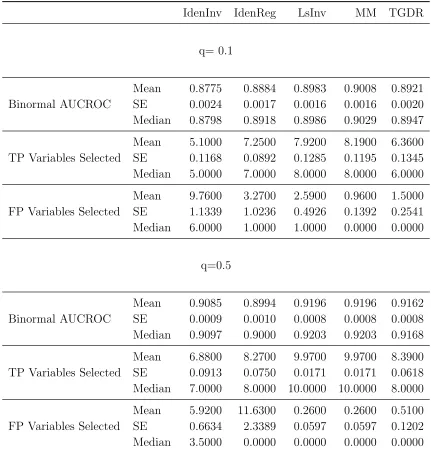
Table 3.1 Equal AR(1) Variance Simulation Performance . . . 48

Table 3.2 Equal Block Variance Simulation Performance . . . 51

Table 3.3 Unequal Block Variance Simulation Performance . . . 55

Table 3.4 Summary of Datasets . . . 57

LIST OF FIGURES

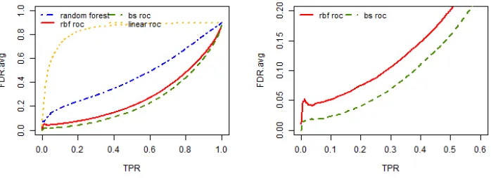
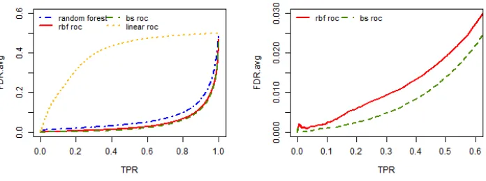
Figure 2.1 Average false discovery rate against the true positive rate out of 200 replicates for all the three simulation settings when the sample size is 400 and the positive example proportion isq= 0.1. The left panels are true positive rate (TPR) on the full range (0,1) while the right panels zoom in to the TPR range of (0, 0.6). . . 29 Figure 2.2 Average false discovery rate against the true positive rate out of 200

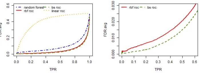
replicates for all the three simulation settings when the sample size is 400 and the positive example proportion isq= 0.5. The left panels are true positive rate (TPR) on the full range (0,1) while the right panels zoom in to the TPR range of (0, 0.6). . . 30 Figure 2.3 Average false discovery rate against the true positive rate out of 200

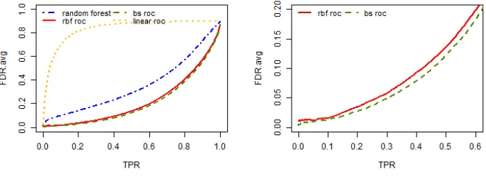
replicates for all the three simulation settings when the sample size is 1000 and the positive example proportion is q = 0.1. The left panels are true positive rate (TPR) on the full range (0,1) while the right panels zoom in to the TPR range of (0, 0.6). . . 31 Figure 2.4 Average false discovery rate against the true positive rate out of 200

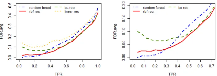
replicates for all the three simulation settings when the sample size is 1000 and the positive example proportion is q = 0.5. The left panels are true positive rate (TPR) on the full range (0,1) while the right panels zoom in to the TPR range of (0, 0.6). . . 32 Figure 2.5 Average false discovery rate against the true positive rate for vertebral

column data set from UCI data repository (Lichman, 2013). The left panel is true positive rate (TPR) on the full range (0,1) while the right panel zooms in to the TPR range of (0, 0.7). . . 33

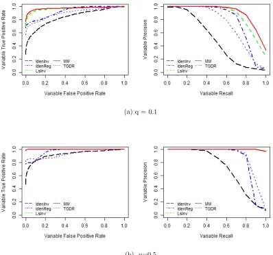
Figure 3.1 Equal AR(1) Variance Simulation ROC Curve and Precision-Recall Curve for Variable Path . . . 49 Figure 3.2 Equal Block Variance Simulation ROC Curve and Precision-Recall

Curve for Variable Path . . . 52 Figure 3.3 Unequal Block Variance Simulation ROC Curve and Precision-Recall

CHAPTER

1

INTRODUCTION

Methods for classification and for variable selection within classification problems have

become increasingly important in the area of statistics and machine learning. The goal

of classification is to predict the category for each unseen object. It usually include two

main phrases. In the training phrase, we have a training set of data, in which we observe

the class and the features for a bunch of objects. Based on the training set with known

classes, classification algorithms seek a model for the class attribute as a function of the

the previously estimated classifier on the new and unseen datasets to determine the class

of each object (Friedman et al., 2001). It is widely used in medical diagnosis, anomaly

detection, information retrieval and various other areas. Variable selection, also known

as feature selection, is the process of identifying and removing redundant or irrelevant

variables, in order to avoid the overfitting problems and thus construct a model with

better performance.

There are many classification algorithms, mainly in five categories summarized by

Kotsiantis et al. (2007). The first group of methods are logic based algorithms, like

deci-sion trees that use a tree-structure graph of decideci-sions to classify the instances (Quinlan,

1986). The second groups are perceptron based algorithms (Rosenblatt, 1962), like

Artifi-cial Neural Networks (ANN) which is composed of many highly interconnected processing

neurones working together to solve the problem (Rumelhart et al., 1985; Zhang, 2000).

The third is statistical learning algorithm which provides a probability that an instance

belongs to a class. Some examples are Linear Discriminant Analysis (LDA) (Friedman,

1989), logistic regression (Cox, 1958), Naive Bayes (Nilsson, 1965), Bayesian Networks

(Jensen, 1996), etc. The fourth is instance-based learning, like k nearest neighbor (kNN)

where an instance is classified by a majority vote of its neighbors (Cover and Hart, 1967).

The last group is the Support Vector Machine (SVM) that tries to find a hyperplane that

separate the two classes with the maximum margin (Burges, 1998). There are also

ensem-ble methods that combine individual classifiers together to achieve a more accurate and

precise system with the cost of increased computation and comprehensibility. Random

Forest is one of the examples that combines many decision trees using an idea of bagging

With all these classifiers described above, one important thing is to measure their

per-formance after the modeling process. A common practice is to use the receiver operating

characteristic (ROC) curve which is highly informative about the classifier performance.

The ROC curve plots the true positive rate (TPR, sensitivity) against the false

posi-tive rate (FPR, 1- specificity ) as the cutoff value is varied. The area under the ROC

curve (AUCROC) is a popular measure of classification accuracy (Hanley and McNeil,

1982). A classifier with a larger area under the ROC curve is often considered to be a

better classifier under the ROC criteria. To calculate the area under the ROC curve

(AU-CROC), there are two main approaches. One is to calculate the area under a parametric

assumption, most common being the binormal assumption. A binormal assumption is to

assume that the decision values of the positive group and the negative group follow two

independent Gaussian distributions (Dorfman and Alf Jr, 1968). The other approach is

to calculate the AUCROC empirically without any distribution assumption.

Instead of using the area under the ROC curve (AUCROC) as a measurement tool

to compare the performance of various classifiers, some have proposed to use the area as

an objective function to obtain a classifier in the first place (Su and Liu, 1993; Liu et al.,

2005; Pepe and Thompson, 2000; Pepe et al., 2006). The problem with these methods

lies in that they either assume a normality for the linear combination of the covariates for

the two groups, which may generate unsatisfactory result for non-normal data, or they

utilize empirical AUCROC which might be unstable and computational intensive.

Although the ROC curve is very useful to measure the classification performance,

when encountering imbalanced data, it might be overly optimistic (Davis and Goadrich,

the ROC curve when facing imbalanced data (Davis et al., 2005; He and Garcia, 2009). It

plots the precision (true discovery rate, TDR) against the recall (true positive rate, TPR)

for various thresholds. Davis and Goadrich (2006) discussed the relationship between the

ROC curve and the Precision-Recall curve. Liu and Bondell (2016) proposed a linear

classifier that maximizes the binormal area under the Precision-Recall curve (AUCPR)

for highly imbalanced data. However, it may perform unsatisfactorily for non-normal

data.

In Chapter 2, we relax the fully parametric assumption, while avoiding the pitfalls

of using the empirical curves. We assume that there exists a transformation function of

the original covariates that makes it follow a binormal distribution. With this relaxed

as-sumption, the classifier no longer needs to be linear, it could take any form of the original

covariates. We then construct the classifier that either maximizes the binormal AUCROC

or maximizes the binormal AUCPR without specifying the form of the transformation

function. Non-parametric functions are employed to approximate the true transformation

function, e.g. B-spline functions and radial basis functions are explored. Empirical

per-formance of the proposed methods is evaluated through several simulation studies and a

real data application.

The classifiers based on maximizing the area under the ROC curve (AUCROC) or the

area under the Precision-Recall curve (AUCPR) discussed above use all of the predictors

to construct the classifiers. However, when redundant or irrelevant variables are used for

constructing the classifier, several problems arise. Firstly, they would cause overfitting

problems and may lead to a worse classifier. Secondly, in some areas like medical diagnosis,

the exact relevant variables helps to get insight into the nature of the problem and makes

the classification model much easier to interpret. Therefore, variable selection within the

classification domain becomes a very important and inevitable task. There exists a lot

of techniques for variable selection, mainly classified in three categories. First is the best

subset selection which compares models with all possible set of predictors and uses criteria

such as cross-validation (Stone, 1974), AIC (Akaike, 1974), and BIC (Schwarz et al., 1978)

to determine the best model. Exhaustive search of all the subsets is very computationally

expensive since the number of subsets to be considered grows rapidly with the number

of predictors. Another group of methods based on forward or backward stepwise variable

selection comes to the rescue. It adds or removes individual predictors in each step, based

on their statistical significance (Hocking, 1976). Tibshirani (1996) pointed out that since

the predictors are either retained or dropped in the model, the model selected can be

very unstable. In other words, small changes in the data may lead to a very different

model being selected. To overcome the limitation inherited in stepwise variable selection,

the third group of methods are developed using regularization techniques to shrink the

coefficients estimates towards zero. Examples include lasso (Tibshirani, 1996) which uses

an l1 penalty to achieve a sparse solution, grouped lasso (Yuan and Lin, 2006; Meier

et al., 2008) where variables are selected in groups, elastic net (Zou and Hastie, 2005)

which uses a combination of l1 and l2 penalty, Dantzig selector (Candes and Tao, 2007)

which is a modification of the lasso, SCAD (Fan and Li, 2001) which is a non-concave

penalty, etc.

In Chapter 3, we incorporate variable selection based on the binormal AUCROC. We

linear or nonlinear transformation (discussed in Chapter 2) of the original covariates in

both groups follow a binormal distribution. We propose three classification and variable

selection methods based on the binormal AUCROC. The first one is estimated through

minimizing the euclidean distance between the sparse coefficients and the dense binormal

AUCROC maximizer with anl1 constraint on the coefficients. The second approach is a

modification of the first one which is based on least square approximation. The third one

utilizes a minorization-maximization (MM) algorithm with coordinate descent to solve a

reformulated problem which is related to the eigenvalue problem. Simulation studies are

conducted in order to evaluate the finite sample performance of the proposed methods.

CHAPTER

2

BINORMAL ROC AND

PRECISION-RECALL CLASSIFICATION

2.1

Introduction

Let Y ∈ {0,1} denote the binary outcome and X = (X1, X2, . . . , Xp)T denote the p

-dimensional vector of covariates. We classify Y = 1 if f(X) ≥ c for some threshold c

estimate the decision function f(X).

Since the area under the ROC curve (AUCROC) can be used as a measurement tool

to compare the performance of various classifiers (Hanley and McNeil, 1982), a very

intuitive way is to use the area as an objective function to obtain a classifier. Many

approaches were proposed for constructing a classifier to improve diagnostic accuracy by

maximizing binormal AUCROC. Su and Liu (1993) proposed to maximize the area under

the ROC curve (AUCROC) so that the best classifier could be achieved under the ROC

criteria. Under the multivariate normality assumption on the original covariates, they

derived the optimal linear combination of these covariates that maximizes the AUCROC.

Liu et al. (2005) derived a linear combination that achieves higher sensitivity over a

certain range of specificity. Hsu and Hsueh (2013) derived a linear combination that

maximizes the binormal partial area under the ROC curve given a pre-specified range.

Ma et al. (2006) proposed a threshold gradient descent algorithm to perform parameter

estimation and variable selection of the linear classifier simultaneously that maximizes the

binormal AUCROC. These methods assume the decision value to be a linear combination

of the original covariates and that they follow the binormal assumption. The binormal

assumption on the linear combination of the covariates are sometimes too strong and

may perform unsatisfactorily when the data follow non-normal distributions.

To relax the parametric distribution assumption, Pepe and Thompson (2000), Pepe

et al. (2006), Ma and Huang (2005) proposed to find the best linear combination for

clas-sification by using the empirical AUCROC as the objective function. While this method

is robust due to its distribution-free assumption, it has two limitations. Firstly, for small

ex-pected AUCROC because of small perturbations. Secondly, for high-dimensional or large

datasets, this empirical optimization process would be quite computationally intensive

(Ma et al., 2006).

Although the ROC curve is a popular tool for measuring classification performance,

the precision recall (PR) curve can expose more differences between classifiers that are not

obvious in ROC space when dealing with highly imbalanced data (Davis and Goadrich,

2006). Davis and Goadrich (2006) studied the relationship between these two curves by

showing that a curve dominates in ROC space if and only if it dominates in PR space.

However, algorithms that optimize the area under the ROC curve do not necessarily

optimize the area under the PR curve (AUCPR). Binormal assumptions on PR curves

were discussed by Brodersen et al. (2010). They showed that the binormal PR curve

outperforms the empirical PR estimates since the latter would be highly imprecise for

the true curve when the sample size is small and data is imbalanced, which ironically is

the situation in which the curve is most useful. Liu and Bondell (2016) proposed a linear

classifier that maximizes the binormal AUCPR for highly imbalanced data. However, it

may perform unsatisfactorily for non-normal data.

In this chapter, we relax the fully parametric assumption, while avoiding the pitfalls

of using the empirical curves. We assume that there exists a transformationT :_Rp →_R

of the original covariates such that T(X) now obeys the binormal assumption. With this relaxed assumption, the classifier no longer needs to be linear, it could take any

form of the original covariates. We then construct the classifier that either maximizes

the binormal AUCROC or maximizes the binormal AUCPR without specifying the form

the true transformation function, e.g. B-spline functions and radial basis functions are

explored in this chapter.

The rest of the chapter is organized as follows. Section 2.2 first reviews the ROC and

the precision-recall curves. Then we describe the details of the binormal model

assump-tion and provide a review of B-splines and radial basis funcassump-tions to be used in fitting.

Section 2.3 provides the estimation details of the proposed methods. Section 2.4 shows

the simulation results for different settings, it also shows the performance of the classifier

when the model assumption is mis-specified. Section 2.5 demonstrates the approach on

vertebral column data and Section 2.6 concludes.

2.2

Methods

2.2.1

Review of ROC and Precision-Recall Curves

Based on the decision function, for every fixed threshold, the confusion matrix can be

constructed as shown in Table 1. True positives (TP) denote instances correctly classified

as positives. False positives (FP) refer to negative instances incorrectly classified as

pos-itive. True negatives (TN) associate with negatives correctly classified as negative. False

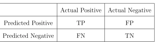
Table 2.1: Confusion Matrix

Actual Positive Actual Negative

Predicted Positive TP FP

Predicted Negative FN TN

In particular, the following threshold-dependent metrics are commonly used.

TPR = T P

T P +F N,

FPR = F P

F P +T N,

Precision = T P

T P +F P,

Recall = T P

T P +F N.

(2.1)

The population versions of the above metrics (2.1) can be written as

TPR(c) =P(f(X)≥c|Y = 1),

FPR(c) =P(f(X)≥c|Y = 0),

Precision(c) =P(Y = 1|f(X)≥c),

Recall(c) =P(f(X)≥c|Y = 1),

(2.2)

for any threshold c.

Given the above quantities, the ROC curve plots the TPR against the FPR as the

(AUCROC) and it is equal to the probability that a classifier will rank a randomly chosen

positive instance higher than a randomly chosen negative one (Bamber, 1975). DefineX0

as a random draw from X|Y = 0, X1 as a random draw from X|Y = 1, then the area

under the ROC curve can be calculated as

AUCROC =P

f(X1)> f(X0)

. (2.3)

Another way to derive the area under the ROC curve is through the integration as

AUCROC =

Z

TPR(c)d{FPR(c)}. (2.4)

However, the derivation is simplified via the representation in (2.3). The Precision-Recall

(PR) curve is a plot of the precision against the recall across different thresholds. A

useful summary of the PR curve is the area under the PR curve (AUCPR) which could

be calculated as

AUCPR =

Z

Precision(c)d{Recall(c)}. (2.5)

2.2.2

Binormal Assumption

We assume that the true decision values are a function of the covariates and follow two

independent Gaussian distributions for the positive and the negative group, which is also

known as the binormal model (Dorfman and Alf Jr, 1968) as follows,

f(X)|Y = 0∼N(ν0, σ20), (2.6)

wheref(·) is a function_Rp _→

R1. The same functionf(·) is applied on both the positive

and the negative groups. Here, the specific form of the functionf(·) does not need to be known and it could take any form of the original covariates. The only assumption is that

there exists such a function that can transform the data into binormal decision values

for the two groups. As long as such function exists, the best classifier can be constructed

by maximizing either the binormal AUCROC or the binormal AUCPR. This assumption

overcomes the strict case of the linear classifier, since the actual decision value may be

2.2.3

Area under the ROC curve and the PR curve

Under the binormal assumption, at any threshold c, we further derive the threshold dependent metrics (2.2) based on the model given in (2.6) and (2.7) as follows,

TPR(c) = P(f(X)≥c|Y = 1)

=P(f(X)−ν1

σ1

≥ c−ν1 σ1

|Y = 1)

= Φ(ν1−c

σ1

),

FPR(c) = P(f(X)≥c|Y = 0)

=P(f(X)−ν0

σ0

≥ c−ν0 σ0

|Y = 0)

= Φ(ν0−c

σ0

),

Precision(c) = P(Y = 1|f(X)≥c)

= P(f(X)≥c|Y = 1)P(Y = 1)

P(f(X)≥c|Y = 1)P(Y = 1) +P(f(X)≥c|Y = 0)P(Y = 0)

=

qΦ(ν1−c

σ1

)

qΦ(ν1−c

σ1

) + (1−q)Φ(ν0 −c

σ0

)

,

Recall(c) = TPR(c) = Φ(ν1−c

σ1

),

(2.8)

where q = P(Y = 1) is the probability of an instance belong to the positive class and Φ(·) denotes the cumulative distribution function of the standard normal distribution.

further derived as

AUCROC = Φ _pν1−ν0

σ2 0 +σ21

!

, (2.9)

AUCPR =

Z

0

qt

qt+ (1−q)Φ

ν0−ν1

σ0

+ σ1

σ0

Φ−1_(t)

dt. (2.10)

In order to compute the AUCROC or the AUCPR under the binormal assumption, we

need to find the values ν0, ν1, σ0, σ1 which are constants that depend on the function,

f(·).

2.2.4

Non-parametric Approximation

To find the unknown function f(X), nonparametric functions are utilized to approxi-mate the true function. This chapter will focus on two types of basis functions, b-spline

functions and radial basis functions, but other choices are possible.

2.2.4.1 B-Spline Functions

In this section, we assume that the true function can be approximated by a combination

of arbitrary functions of the covariates and the contribution of each covariate is additive.

This is the so-called additive model first suggest by Buja et al. (1989). The function of

each covariate is further specified to be a combination of b-splines where a b-spline is a

f(X)≈ p

X

i=1

gi(Xi), (2.11)

where gi(Xi) =

PK

j=1βijBj,m(Xi). Here,Bj,m is the jth b-spline function of order m. For

simplicity, we set the order for the basis expansion to m = 4 which leads to the cubic spline functions. For simplicity, the number of basis functions is assumed to be the same

for each variable. The number of basis functions K for each variable is then the only tuning parameter in this model.

2.2.4.2 Radial Basis Functions

An alternative approach to approximate a given function is to use a set of radial basis

functions (RBF). Since the RBF approach is based on the distance from a covariate

vector to a given knot location, it implicitly includes the interactions between the full set

of covariates, rather than an additive model. The approximation function is represented

as a sum ofK radial basis functions with form

f(X)≈ K

X

i=1

βihi(X), (2.12)

wherehi(X) = exp

||X−Xc(i)||2

ρ is thei

th_{radial basis function associated with thei}th_center

Xc(i). Each of the radial basis functions is weighted by an appropriate coefficientβi. Each

covariate is normalized to have mean 0 and variance 1 before performing the radial basis

function transformation. A k-means clustering method is used to find the clusters and

the center points with a pre-specified number of centers based on the normalized data.

2.3

Estimation

Under the binormal assumption, the best classifier in terms of ROC criteria is obtained

by maximizing the area under the ROC curve, the best classifier regards to PR criteria

is obtained by maximizing the area under the PR curve.

After the nonparametric approximation, we get a set of transformed variables Z =

(Z1(X), . . . , ZL(X))T where Z are (Bj,m(Xi))_{i=1,...,p,j=1,...,K} for the b-spline

transfor-mation and (hj(X))_j=1,...,K for the radial basis function transformation. The binormal

assumption could then be rewritten as

ZTβ|Y = 0∼N(ν0, σ20), (2.13)

ZTβ|Y = 1∼N(ν1, σ21), (2.14)

where β ∈ _RL _{denotes the corresponding coefficients which need to be estimated. Note}

that L=K for the radial basis functions, andL=pK for the B-splines.

We further assume that Z has mean µ₀ and variance Σ0 for group Y = 0, and has

meanµ₁ and varianceΣ1 for groupY = 1. Defineµ0 with entriesµ0j =E[Zj(X)|Y = 0]

andµ₁with entriesµ1j =E[Zj(X)|Y = 1]. DefineΣ0such that Σ0jk = Cov [Zj(X), Zk(X)|Y = 0],

define Σ1 such that Σ0jk = Cov [Zj(X), Zk(X)|Y = 1].

The binormal AUCROC and AUCPR would then be calculated based onµ₀,µ₁,Σ0,Σ1,β

so that ν0 =µ0β, ν1 =µ1β,σ02 =β

T_Σ

0β, and σ12 =β

T_Σ

2.3.1

Estimation using AUCROC

After the nonparametric approximation, the binormal AUCROC in (2.9) is then given

by

AUCROC(β) = Φ

 

(µ₁−µ₀)Tβ

q

βT(Σ0+Σ1)β



, (2.15)

where Φ is the standard normal cumulative distribution function and β, µ₀,µ₁,Σ0,Σ1

are specified previously.

To maximize (2.15) , it is equivalent to maximizing (µ1−µ0)

T_β

q

βT(Σ0+Σ1)β

, since Φ is a

monotone increasing function. Furthermore, up to a change in sign, it is the same as

maximizing the squared form β

T

(µ₁−µ₀)(µ₁−µ₀)T_β

βT(Σ0+Σ1)β

, which is a generalized

eigen-value problem and could be solved directly with the closed-form solution as

β_ROC = argmax β

{AUCROC(β)} ∝(Σ0+Σ1)−1(µ1−µ0). (2.16)

We then estimate β_ROC by plugging in the sample version, to obtain

ˆ

β_ROC = argmax β

{AUCROC(\ β)} ∝( ˆΣ0+ ˆΣ1)−1( ˆµ1−µˆ0), (2.17)

where ˆµ₀,µˆ₁,Σˆ0,Σˆ1 are the sample mean and the sample covariance of the transformed

2.3.2

Estimation using AUCPR

After the nonparametric approximation, the binormal AUCPR in (2.10) can be rewritten

as

AUCPR(β) =

Z

0

qt

qt+ (1−q)Φ

"

(µ₀−µ₁)T_β

p

βTΣ0β

+

p

βTΣ1β

p

βTΣ0β

Φ−1_(t)

#dt,(2.18)

where Φ is the standard normal cumulative distribution function, Φ−1_{is the inverse of the}

standard normal cumulative distribution function,q =P(Y = 1) is the probability of an instance belonging to the positive class. We plug in the sample versions, ˆµ₀,µˆ₁,Σˆ0,Σˆ1,

and would like to construct a classifier that maximizes this area, which is

ˆ

β_PR = argmax β

{AUCPR(\ β)}. (2.19)

Note that, if we had assumedΣ0 andΣ1 to be equal or proportional, then maximizing

AUCPR would be equivalent to minimizing (µ0 −µ1)

T_β

p

βTΣ0β

, which leads to the optimal

classifier with the form ˆΣ−₀1( ˆµ₁−µˆ₀). So under this assumption, the solution would be

proportional to the maximizer for AUCROC. However, this assumption is too strong and

it is difficult to even envision to be true in reality since Σ0,Σ1 are the variances for the

transformed variablesZ. Therefore, we seek the solution without the assumption of equal

variance via a numerical method.

A gradient descent algorithm with backtracking line search is applied to this problem.

less computational cost than choosing an infinitesimal step size , e.g. s = 1× 10−4_.

Instead of only moving an infinitesimal amount along the search direction, performing

the line search allows us to start moving a relatively large step size along the direction

and if needed it will iteratively shrink the step sizes until the criterion is met. It is more efficient since one can move a larger amount without worry about moving too far to miss

the local optimum by iteratively shrinking the step size. The full algorithm is given by

Algorithm 1.

We compute the derivative of AUCPR with respect to β as follows,

dAU CP R

dβ =

Z

0

−qt

qt+ (1−q)Φ

"

(µ₀−µ₁)Tβ p

βTΣ0β

+

p

βTΣ1β p

βTΣ0β

Φ−1_(t)

#!2 ×(1−q)

×φ

"

(µ₀−µ₁)Tβ p

βTΣ0β

+

p

βTΣ1β p

βTΣ0β

Φ−1(t)

#

×





µ₀−µ₁ p

βTΣ0β

+ Φ

−1_(t)Σ1β p

βTΣ0β p

βTΣ1β

−(µ0−µ1)

T_βΣ0β

q

(βTΣ0β)3

−Φ

−1_(t)p

βTΣ1βΣ0β q

(βTΣ0β)3 

dt

(2.20)

Algorithm 1 describes the details about the implementation of the gradient descent

algorithm. For classification purpose, both the AUCROC and the AUCPR estimators are

only identifiable up to a scale constant. That is, instead of the absolute magnitude of β,

only the direction of β, which represent the relative effects, can be estimated from the

AUCROC and AUCPR objective function. For identifiability, we introduce an anchor

variable whose estimated coefficient is set to a constant. Without loss of generosity, for

for the radial basis function transformation, we assume the feature associated with the

center surrounded by the largest number of observations as the anchor; for the linear

classifier, we assume the first variable to be the anchor. Since the objective AUCPR is

not a convex function, only a local maximum would be achieved with a specific starting

value. Thus, different initial values need to be tried and the one with the largest AUCPR

would be the final solution. In our method, we use three initial values as β_initial, (1) all

zeros but the anchor are set to 1, (2) all zeros but the anchor are set to -1, (3) the

Algorithm 1 Gradient Descent for Maximizing AUCPR

1: β(0) ←β_initial

2: while iter < maxiterdo

3: Compute the gradient gd= dAU CP R_dβ . Denote the jth component of gd asgd_j.

4: Make gdanchor= 0, then if maxj{|gdj|}= 0, stop the iterations.

5: begin backtracking line search with initial step size s

6: while siter < smaxiter do

7: βtemp ←β(iter)+s×gd

8: Compute AUCPRtemp based on βtemp

9: if AUCPRtemp ≤ AUCPR(iter) then

10: s←s/2

11: siter ← siter+1

12: else

13: break

14: end if

15: end while

16: end line search

17:

18: β(iter)←βtemp

19: AUCPR(iter)←AUCPRtemp

20: if |AUCPR(iter)−AUCPR(iter-1)|<tol×AUCPR(iter-1) then

21: break

22: end if

23: iter ← iter+1 24: end while

25: return βˆ =β(iter)

26:

27: Use a differentβ_initial, repeat steps 1-24.

2.3.3

Tuning Parameter Selection

For b-spline approximation, the number of basis functions K for each variable is the tuning parameter. For radial basis function approximation, the number of centersK and the scale parameter ρ are the tuning parameters. In our numerical studies, we propose using theV-fold cross validation (CV) to choose the tuning parameters. For a pre-defined integer V, we randomly partition the data into V complementary subsets of equal sizes. For estimation using AUCROC, we select the tuning parameters that maximize the ROC

CV score as

ROC CV Score = 1

V V

X

i=1

\

AUCROC(i)

ˆ

β(_ROC−i)

, (2.21)

where ˆβ(_ROC−i) is the estimated coefficient without the samples in thei-th fold andAUCROC\ (i)

is the binormal AUCROC estimator with the data in the i-th fold. For estimation using AUCPR, we choose the tuning parameters to maximize the PR CV score given by

PR CV Score = 1

V V

X

i=1

\

AUCPR(i)βˆ(_PR−i), (2.22)

where ˆβ(_PR−i) is the estimated coefficient without the data in the i-th fold and AUCPR\ (i)

is the binormal AUCPR estimator with the data in thei-th fold.

2.4

Simulation Study

In this section, we conduct several simulations with 200 replicates each to assess the

the AUCPR. In each simulation, we generate a training sample to fit the model and

a separate test set of size 10000 to compare the performance for different classifiers.

For methods utilizing radial basis functions and b-spline functions, we conduct a 5-fold

cross validation as described in Section 2.3.3 on the training sample to determine the

best tuning parameters. The coefficients would then be estimated on the whole training

data using the best tuning parameters. For other methods, we estimate the coefficients

directly on the whole training data. Three benchmark methods are used for comparison

purposes. Two are linear classifiers maximizing the binormal AUCROC, and the binormal

AUCPR, respectively. The third is Random Forests, a very popular ensemble method for

classification.

We experiment different combinations of the training sample size and the proportion of

positive examples. Training sample size of 400 and 1000 are considered. Both imbalanced

case with q = 0.1 and balanced case withq = 0.5 are considered. For each combination, we consider three different settings such that the true function f(x) includes some of the four following pieces, 10x2

1, 5 log(x2), exp(x3), 10 log(x2) exp(x3) in each setting. The

first three pieces represent the main effect and the last piece represents the interaction

between variables.

2.4.1

Setting 1: Binormal Additive Data

Given y= 0, we generate f(x)∼N(46,22_{). Given y= 1, we generate f(x)∼N(51,2}2_).

Letf(x) = 10x2₁+5 log(x2)+exp(x3). First we generatex3so that exp(x3)∼Uniform(10,15),

then we generate x2 so that log(x2)∼ Uniform

0,f(x)−exp(x3)

5 + exp(x3)

, lastly we generate

x1 such thatx21 =

f(x)−5 log(x2)−exp(x3)

classi-fiers will not depend on variablex3 much sincex3is generated from the same distribution

for both the positive and the negative group.

The average false discovery rate (FDR) against the true positive rate (TPR) out of

200 replicates are shown in Figure 2.1(b), Figure 2.2(b), Figure 2.3(b), Figure 2.4(b).

Each represents training sample size of 400 and positive example proportion of 10%,

training sample size of 400 and positive example proportion of 50%, training sample size

of 1000 and positive example proportion of 10%, training sample size of 1000 and positive

example proportion of 50%, respectively.

For each TPR, a lower false discovery rate is desired. The results of the AUCPR

classifier is similar to the AUCROC classifier and are not shown here. In all the different

combinations of the sample size and the positive example proportions, our proposed

classifiers, both the AUCROC classifier and the AUCPR classifier are able to find the

optimal classifier close to the truth and they outperform both the linear classifiers and the

random forest method in terms of false discovery rate (FDR). The linear classifiers have

the worst performance, since they reach high FDR very quickly and have higher FDR

than all the other methods. This is expected, since the simulation data are nonlinear, so

that the fully parametric linear classifiers fail to capture the true decision value function.

The random forest classifier performs better than the linear classifier since it does not

make any distribution assumption for the data. Nevertheless, it does not capture the

nonlinear decision boundary well and is still worse than our proposed methods.

When changing from an imbalanced case (q = 0.1) to a balanced case (q = 0.5), or the sample size becomes larger, the classification problem becomes easier. Hence all

superiority of our proposed method upon others becomes less severe.

The b-spline approximation is slightly better than the radial basis function here in

terms of FDR. In this setting, the true function is an additive model, and the b-spline

ap-proximation is good enough to capture this while the radial basis function apap-proximation

is more complex and not necessary.

For either of the nonparametric approximation, the performance of the AUCROC

maximizer and the AUCPR maximizer are very similar. Although in theory, when data

are highly imbalanced, the PR curve is better than the ROC curve and can show much

more differences when comparing various classifiers, the AUCPR maximizer has very

sim-ilar performance with the AUCROC maximizer since the AUCPR maximizer is achieved

by numerical algorithm after nonparametric approximation and would have more

uncer-tainty introduced.

2.4.2

Setting 2: Binormal Interactive Data

We consider the same binormal distribution as in the setting 1. Given y = 0, we generate f(x) ∼ N(46,22). Given y = 1, we generate f(x) ∼ N(51,22). Here, a different transformation function f(·) is considered. Let f(x) = 10x2

1 + 5 log(x2) +

exp(x3) + 10 log(x2) exp(x3) which includes interaction between x2 and x3. We first

gen-erate x3 such that exp(x3) ∼ Uniform(10,15), then generate x2 such that log(x2) ∼

Uniform

0,f(x)−exp(x3)

5 + 10 exp(x3)

, lastly we generatex1 such that x21 =

f(x)−5 log(x2)−

exp(x3)−10 log(x2) exp(x3)

/10. Compared to setting 1, setting 2 considers the case where variables have interaction with each other rather than a simple additive model.

10 log(x2) exp(x3) is significantly different for the two groups.

The performance of the proposed classifiers and the other underlying classifiers are

shown in Figure 2.1(b), Figure 2.2(b), Figure 2.3(b), Figure 2.4(b). Each represents

train-ing sample size of 400 and positive example proportion of 10%, traintrain-ing sample size of

400 and positive example proportion of 50%, training sample size of 1000 and positive

example proportion of 10%, training sample size of 1000 and positive example proportion

of 50%, respectively.

The results are mostly similar as setting 1 with our proposed classifiers being the

best. The difference lies in that the radial basis function approximation is better than

the b-spline approximation. This is due to the fact that the true model has interaction

between variables, and radial basis functions are designed to capture this while the

b-spline approximation is not.

2.4.3

Setting 3: Non-normal Interactive Data

Setting 1 and setting 2 both consider the situations where the binormal assumption is

correct. However, the performance of the proposed method under the cases where the

model is mis-specified is also of interest. In setting 3, we let the true function follow

two different shifted Gamma distribution for the two groups. Given y = 0, we generate

f(x) ∼ Gamma(2,1) + 30. Given y = 1, we generate f(x) ∼ Gamma(8,1) + 30. We consider the same transformation function f(·) which includes interaction between the variables as in setting 2 and uses the same generation scheme forx1,x2, x3 as in setting

2.

3. Each represents training sample size of 400 and positive example proportion of 10%,

training sample size of 400 and positive example proportion of 50%, training sample size

of 1000 and positive example proportion of 10%, training sample size of 1000 and positive

example proportion of 50%, respectively. We can see that when the binormal assumption

is seriously violated as in setting 3, the proposed methods still give very satisfactory

performance which is better than the random forest method and the linear classifiers.

2.5

Application to Vertebral Column Data

We applied our methods on the vertebral column data from the UCI data repository

(Lichman, 2013). The data consists of 310 records with 210 abnormal patients and 100

normal patients. Each patient has six biomechanical attributes derived from the shape

and orientation of the pelvis and lumbar spine which are pelvic incidence, pelvic tilt,

lumbar lordosis angle, sacral slope, pelvic radius and grade of spondylolisthesis.

The data are randomly split into two parts, 75% training and 25% testing. A

5-fold cross validation is conducted on the training set for the methods using radial basis

functions and b-spline approximation. The partition process is repeated 50 times. Average

false discovery rate out of the 50 testing data sets is plotted in Figure 2.5. The AUCPR

classifiers have very similar performance with the AUCROC classifiers and are not shown

in the plot. It can be seen that the AUCROC maximizer with the radial basis function

approximation is the best among the methods in terms of FDR. Although random forest

is a bit better when TPR is smaller than 0.3, the improvement is very little and we could

always choose a cutoff value with a lot higher TPR without much sacrifice in the FDR,

(a) Setting 1: Binormal non-interactive data

(b) Setting 2: Binormal interactive data

(a) Setting 1: Binormal non-interactive data

(b) Setting 2: Binormal interactive data

(c) Setting 3: Non-normal interactive data

(a) Setting 1: Binormal non-interactive data

(b) Setting 2: Binormal interactive data

(a) Setting 1: Binormal non-interactive data

(b) Setting 2: Binormal interactive data

(c) Setting 3: Non-normal interactive data

better than the b-spline approximation likely due to strong interactions between these

covariates.

Figure 2.5: Average false discovery rate against the true positive rate for vertebral col-umn data set from UCI data repository (Lichman, 2013). The left panel is true positive rate (TPR) on the full range (0,1) while the right panel zooms in to the TPR range of (0, 0.7).

2.6

Conclusion

In this chapter, we propose using the binormal AUCROC and the binormal AUCPR as

the objective function for binary classification using a nonparametric approximation of

the true decision value function. Both simulation studies and real data application show

that the proposed methods outperform linear classifiers and random forest classifiers.

The proposed methods have a very flexible assumption that only assumes the existence

than the fully parametric assumption in the linear classifier. When this assumption is

seriously violated, the proposed methods still give very satisfactory performance which

is better than the random forest method and the linear classifier.

When there is a strong interaction, the radial basis function approximation would

lead to better results. When the truth is an additive model, the b-spline approximation

would be suggested. Other nonparametric approximations can also be explored according

CHAPTER

3

BINORMAL ROC CLASSIFICATION

AND VARIABLE SELECTION

3.1

Introduction

Variable selection, also known as feature selection, is the process of identifying and

remov-ing redundant or irrelevant variables. When redundant or irrelevant variables are used

overfit-ting problems and may lead to a worse classifier. Secondly, in some areas like medical

diagnosis, which variables are import for the disease diagnosis is of big interest. Thirdly,

knowing the exact relevant variables helps to get insight into the nature of the problem

and makes the classification model much easier to interpret. Therefore, variable selection

within the classification domain becomes a very important task.

Recall that the classification problem consists of a binary response Y ∈ {0,1} and a p-dimensional vector of covariates X = (X1, X2, . . . , Xp)T. In this chapter, rather

than making a binormal assumption on any general transformation f(X) as discussed in Chapter 2, we consider a specific case where f(X) being βTX follows the binormal distribution where β is the corresponding coefficients that need to be estimated. In

ad-dition, we consider the decision function f(X) to be “linear risk scores” βTX. The goal here is to estimateβ.

To incorporate variable selection based on binormal AUCROC, Ma et al. (2006)

pro-posed a threshold gradient descent algorithm to perform parameter estimation and

vari-able selection of the linear classifier simultaneously that maximizes the binormal

AU-CROC. Yu and Park (2014) proposed a l1 penalized regression estimator based on the

binormal AUCROC.

In this chapter, we propose three classification and variable selection methods that

are based on the binormal AUCROC. The first one is estimated through minimizing

the euclidean distance between the sparse coefficients and the dense binormal AUCROC

maximizer with an l1 constraint on the coefficients. The second approach is a

modifi-cation of the first one which is based on least squares approximation. The third one

a reformulated problem which is related to the eigenvalue problem.

The rest of the chapter is organized as follows. Section 3.2 provides the details of

the binormal model assumption and the binormal AUCROC. Section 3.3 illustrates the

proposed classification and variable selection methods. Simulation results for different

settings are provided in Section 3.4 and real data application results are shown in Section

3.5. Section 3.6 concludes.

3.2

Preliminaries

3.2.1

Binormal Assumption

Use the binormal assumption on f(X) given in (2.6) and (2.7), we consider a specific case with f(X) =βTX. We have

βTX|Y = 0∼N(ν0, σ20), (3.1)

βTX|Y = 1∼N(ν1, σ21). (3.2)

Notice that the normality of X itself is not necessary, we only require the linear

combi-nation of X to be normal, which is more likely to hold.

3.2.2

Area under the ROC curve

Define X|Y = j to have mean µj = E(X|Y = j) and variance Σj = Var(X|Y = j)

under the ROC curve in (2.9) can be further derived as

AUCROC(β) = Φ

 

βT(µ₁−µ₀)

q

βT(Σ0+Σ1)β



, (3.3)

where Φ is the standard normal cumulative distribution function.

3.3

Classification and Variable Selection Methods

Xu and Bondell (2016) proved that maximizing (3.3), up to a change in sign, is the same

as maximizing the squared form,

βT(µ₁ −µ₀)(µ₁−µ₀)Tβ βT(Σ0+Σ1)β

, (3.4)

which is a generalized eigenvalue problem and that can be solved directly with closed-form

solution

β_ROC = argmax β

{AUCROC(β)} ∝(Σ0+Σ1)−1(µ1−µ0), (3.5)

up to a change in sign. We then estimate β_ROC by plugging in the sample version, to

obtain

ˆ

β_ROC = argmax β

{AUCROC(\ β)} ∝( ˆΣ0+ ˆΣ1)−1( ˆµ1−µˆ0), (3.6)

where ˆµ₀,µˆ₁,Σˆ0,Σˆ1 are the sample mean and the sample covariance of the predictors

X for the two groups.

The dense solution ˆβ_ROCutilizes all the covariates available without doing any variable

variables are used. Therefore, we study to perform the variable selection and classification

simultaneously by optimizing the binormal AUCROC.

Throughout the chapter, for a vector q = (q1, ..., qp)T ∈ Rp, define the l1 norm as

kqk1 =

Pp

i=1|qi|,l2norm askqk2 =

pPp

i=1qi2. We propose several approaches to achieve

the variable selection goal.

3.3.1

Method 1: IdenInv

The intuitive way of getting a sparse solution but as accurate as the dense solution ˆβ_ROC

is to minimize the euclidean norm between these two solutions with a lasso penalty given

by

β= argmin β

n

kβ−( ˆΣ0+ ˆΣ1)−1( ˆµ1−µˆ0)k 2

2+λkβk1

o

, (3.7)

where λ ≥ 0 is the tuning parameter that controls the sparseness of the coefficients. When λ= 0, the solution is exactly the same as the dense solution ˆβ_ROC. If λ increases, some elements of β are exactly zero, thus we get a more sparse solution. To solve (3.7),

one can use a trick, that is to treat ( ˆΣ0+ ˆΣ1)−1( ˆµ1−µˆ0) as the response, and create an

identity matrix Ip ∈Rp×p as the design matrix for the independent variables. Then the

LARS algorithm (Efron et al., 2004) can be utilized to get the whole solution path with

3.3.2

Method 2: LsInv

The IdenInv method does not account for the variance of ˆβ_ROC. However, using the

variance of ˆβ_ROC would lead to a more efficient estimator. Therefore, we would like to

take care of the variance of ˆβ_ROC. Since the direct variance of ˆβ_ROC is hard to

com-pute, we consider ˆβ∗_ROC = (Σ0 +Σ1)−1( ˆµ1 −µˆ0), whose variance can be calculated as

V = Var( ˆβ∗_ROC) = (Σ0+Σ1)−T(

Σ0

n0

+ Σ1

n1

)(Σ0 +Σ1)−1. Now utilizing the least square

approximation, we have

β = argmin β

n V

−1/2_βˆ∗

ROC−V

−1/2_β

2 2

+λkβk1

o

. (3.8)

where V−1 is the inverse of V that can be decomposed into V−1 = V−1/2V−1/2, and

λ≥0 is the tuning parameter that controls the sparseness of the coefficients β. We call this method “LsInv’ since it utilizes the idea of least squares approximation and ˆβ∗_ROC,

which requires an inverse step.

The LsInv method uses a more accurate objective to solve, which leads to a more

accurate sparse solution β than the IdenInv method. When solving (3.8), we use ˆV =

( ˆΣ0+ ˆΣ1)−T(

ˆ Σ0 n0 + ˆ Σ1 n1

)( ˆΣ0+ ˆΣ1)−1 to estimateV and use a similar trick as in IdenInv.

We treat ˆV−1/2βˆ∗_ROC as the response and ˆV−1/2 as the design matrix, then employ the

LARS algorithm (Efron et al., 2004) to get the whole solution path with different λ

3.3.3

Method 3: MM

Now instead of dealing with ˆβ_ROC in various ways, we take a step back and consider the

generalized eigenvalue problem (3.4) directly, which is equivalent to

MaximizenβTAβo subject toβTW β ≤1, (3.9) where A= (µ₁−µ₀)(µ₁−µ₀)T _{and W = (Σ}

0+Σ1). We define the penalized problem

as

β = argmax

β

n

βTAβ−λkβk1

o

subject to βTW β ≤1 (3.10)

whereA= (µ₁−µ₀)(µ₁−µ₀)T _{, W = (Σ}

0+Σ1) and λ≥0 is a tuning parameter. We

can utilize the minorize-maximization (MM) algorithm to solve the problem (Lange et al.,

2000; Hunter and Lange, 2004; Lange, 2004). It tries to find a surrogate function that

minorizes the objective function and then optimizes the surrogate function iteratively to

drive the objective function upward towards the maximum. In each iteration, we consider

two scenarios. When W is a diagonal matrix, the problem is easier and each coefficient

can be updated separately in each iteration (Gaynanova et al., 2016). When W is a

symmetric but not diagonal matrix, a coordinate descent algorithm is employed in each

iteration. A detailed proof is provided in the Appendix. The Algorithm details are shown

Algorithm 2

1: β(1) ←β_initial

2: repeat

3: m ←1

4: if W is diagonal matrix then

5: for i= 1,2, . . . , p do

6: di ← ST

(Aβ(m))_i

wii , λ

2wii

where wii is the ith is diagonal element of W

and

7: (Aβ(m))i is the ith element of Aβ(m).

8: end for

9: else if W is symmetric but not diagonal matrix then

10: repeat

11: d(1) ←dinitial

12: k ←1

13: for i= 1,2, . . . , p do

14: d(_ik+1) ←ST(Aβ

(m)

)i−(d(k))T−iW−i

wii ,

λ

2wii

15: where d(₋k_i)= (d₁(k+1),· · · , d(_i−k+1)₁ , d(_ik₊₁),· · ·d(pk)),

16: and W−i = (w1i,· · · , wi−1,i, wi+1,i,· · · , wpi).

17: end for

18: g(d(k+1))←(d(k+1))TW d(k+1)−2(d(k+1))TAβ(m)+λkd(k+1)k1

19: k ←k+ 1

20: untilk =kmax or|g(d(k+1))−g(d(k))|< |g(d(k))|

21: end if

22: if d6=0 then

23: β(m+1) ←d/(dTW d)12

24: else

25: β(m+1) ←0

26: end if

27: h(β(m+1))←(β(m+1))T_Aβ(m+1)_−λk

β(m+1)k1

3.4

Simulation

In this section, we conduct several simulations to assess the finite sample performance of

the proposed classification and variable selection methods. In each setting, we generate

a training sample of size 1000 to fit the model, a separate validation set of size 1000 to

find the optimal tuning parameters and finally a test set of size 1000 to compare the

performance for different methods. The process is repeated 100 times for each simulation

setting.

Three benchmark methods are used for comparison purposes. The first method by

Yu and Park (2014) has objective argmin_β{k( ˆΣ0 + ˆΣ1)β − ( ˆµ1 − µˆ0)k2 + λ

P

|βj|}.

We denote it as “IdenReg”. The second is the threshold gradient descent regularization

(TGDR) method discussed in Ma et al. (2006). For all the ROC related methods, e.g.

our proposed methods and TGDR, we choose the tuning parameters that maximize the

AUCROC in the validation set.

In these simulations, we will generate predictorsX|Y =j from a multivariate normal distribution with mean µj and covariance Σj in all settings. Following the proof from

Liu and Bondell (2016) using Neyman-Pearson lemma, we can show that the optimal

risk score function is

XT(Σ−₀1 −Σ−₁1)X+ 2(Σ₁−1µ₁−Σ−₀1µ₀)TX. (3.11)

If we assume Σ0 and Σ1 are equal or proportional to each other, then the optimal risk

score function is linear in X, with coefficients β ∝(Σ0 +Σ1)−1(µ1−µ0). Otherwise, if

be quadratic.

Let q = P(Y = 1) be the probability of an instance belonging to the positive class. For each simulation setting, we consider both q = 0.1 representing the imbalanced data case and q = 0.5 representing the balanced case. Define 0k ∈ Rk as a vector of length k

with all elements equal to 0. Similarly, define 1k ∈ Rk as a vector of length k with all

elements equal to 1. Define 0k×l ∈Rk×l as a matrix with k rows and l columns with all

elements equal to 0.

When assessing the performance of the variable selection process, we will use the

fol-lowing quantities and plots. For a model with a specific number of variables, the variable

true positive rate (Variable TPR, Variable Recall) measures the proportion of important

variables that are correctly identified. The variable false positive rate (Variable FPR)

measures the proportion of unimportant variables that are incorrectly identified as

im-portant. The Variable Precision represents the proportion of detected important variables

that are truly important. Knowing the order of the variables that come into the model, we

can construct the ROC curve for the variable path which plots the Variable TPR against

the Variable FPR as the number of variables in the model is varied. The Precision-Recall

curve for the variable path plots the Variable Precision versus the Variable Recall when

3.4.1

Simulation Setting 1: Equal AR(1) Variance Model

For a vector of pvariables, an AR (1) covariance matrix Σ∈_Rp×p _{has the structure of}

Σ=σ2(ρ|i−j|) = σ2

           

1 ρ ρ2 _{. . . ρ}p−1

ρ 1 ρ . . . ρp−2

ρ2 _{ρ 1 . . . ρ}p−3

..

. ... ... . .. ...

ρp−1 ρp−2 ρp−3 . . . 1

           

p×p

, (3.12)

whereρ is the AR(1) correlation parameter andσ2 _{is the variance. Kac et al. (1953) has}

shown that the inverse of the AR(1) covariance is given by

Σ−1 = 1

σ2_(1−ρ2₎

                1 −ρ

−ρ 1 +ρ2 _−ρ

−ρ . .. ...

. .. ... . ..

. .. 1 +ρ2 _−ρ

−ρ 1                

p×p

. (3.13)

Let µ₀ = 0500, µ1 = (0,18,0,0490). Let Σ0 = Σ1 = (0.5|i−j|)500×500. Σ0 and Σ1 are

equal and they follow the AR(1) variance structure withσ2 _{= 1 andρ= 0.5. Giveny= 0,}

we generate X ∼M N(µ₀,Σ0). Given y= 1, we generate X ∼M N(µ1,Σ1). According

to the best risk score function (3.11), the optimal linear risk score function is linear inX1

equal variance. Hence, we have 10 true important variablesX1 throughX10and the other

490 unimportant variables do not contribute to the classifier in any way. Notice that the

mean for the positive group and the negative group only differ in X2 through X8. In

other words, if one performs variable screening marginally by t-tests, one would fail to

detectX1 andX10as important variables. This leads to an interesting thing to see about

our proposed methods.

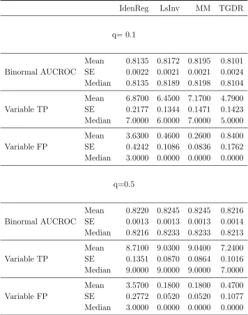
For both the imbalanced case (q = 0.1) and the balanced case (q = 0.5), Table 3.1 summarizes the AUCROC on the test data sets across 100 replicates. It also summarizes

the number of important variables selected (Variable TP) and the number of unimportant

variables selected (Variable FP) when using the best tuning parameter. On the other

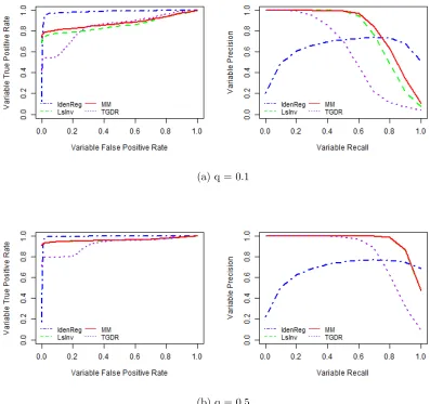
hand, Figure 3.1 plots the ROC curve and the Precision-Recall curve for the variable

selection paths. When data are imbalanced and q = 0.1, our proposed method MM achieves the highest average binormal AUCROC on the test set across 100 replicates

and it is significantly better than TGDR, IdenReg, IdenInv. The other proposed method

LsInv is comparable to MM in terms of the AUCROC but is worse than MM in variable

selection. It can be seen that MM selects a significantly larger number of true important

variables and significantly smaller number of unimportant variables when compared with

LsInv. Figure 3.1(a) shows that MM has the best variable selection path, following by

LsInv, IdenReg, TGDR, IdenInv, sequentially. When q = 0.5, our proposed methods LsInv and MM have very similar outcomes and they both outperform other methods.

LsInv and MM are able to select all of the important variables including marginally

undetectable variables X1 and X10 with nearly no unimportant variables selected. In

other methods like IdenInv, IdenReg and TGDR. The IdenInv estimator always performs

the worst and thus we will not show its results in the later simulations and real data

Table 3.1: Equal AR(1) Variance Simulation Performance

IdenInv IdenReg LsInv MM TGDR

q= 0.1

Binormal AUCROC

Mean 0.8775 0.8884 0.8983 0.9008 0.8921

SE 0.0024 0.0017 0.0016 0.0016 0.0020

Median 0.8798 0.8918 0.8986 0.9029 0.8947

TP Variables Selected

Mean 5.1000 7.2500 7.9200 8.1900 6.3600

SE 0.1168 0.0892 0.1285 0.1195 0.1345

Median 5.0000 7.0000 8.0000 8.0000 6.0000

FP Variables Selected

Mean 9.7600 3.2700 2.5900 0.9600 1.5000

SE 1.1339 1.0236 0.4926 0.1392 0.2541

Median 6.0000 1.0000 1.0000 0.0000 0.0000

q=0.5

Binormal AUCROC

Mean 0.9085 0.8994 0.9196 0.9196 0.9162

SE 0.0009 0.0010 0.0008 0.0008 0.0008

Median 0.9097 0.9000 0.9203 0.9203 0.9168

TP Variables Selected

Mean 6.8800 8.2700 9.9700 9.9700 8.3900

SE 0.0913 0.0750 0.0171 0.0171 0.0618

Median 7.0000 8.0000 10.0000 10.0000 8.0000

FP Variables Selected

Mean 5.9200 11.6300 0.2600 0.2600 0.5100

SE 0.6634 2.3389 0.0597 0.0597 0.1202

Median 3.5000 0.0000 0.0000 0.0000 0.0000

(a) q = 0.1

(b) q=0.5

Figure 3.1: Equal AR(1) Variance Simulation ROC Curve and Precision-Recall Curve for Variable Path

3.4.2

Simulation Setting 2: Equal Block Variance Model