A Robust and Efficient Finite Volume method for Compressible Two-Phase Flows at All Speeds on Unstructured Grids.

(1)

ABSTRACT

PANDARE, ADITYA KIRAN. A Robust and Efficient Finite Volume method for Compressible Two-Phase Flows at All Speeds on Unstructured Grids. (Under the direction of Dr. Hong Luo).

(2)

(3)

A Robust and Efficient Finite Volume method for Compressible Two-Phase Flows at All Speeds on Unstructured Grids

by

Aditya Kiran Pandare

A dissertation submitted to the Graduate Faculty of North Carolina State University

in partial fulfillment of the requirements for the Degree of

Doctor of Philosophy

Aerospace Engineering

Raleigh, North Carolina

2018

APPROVED BY:

Jack Edwards Jr. Pramod Subbareddy

Pierre Gremaud Hong Luo

(4)

DEDICATION

(5)

BIOGRAPHY

(6)

ACKNOWLEDGEMENTS

First and foremost, I would like to thank my advisor Dr. Hong Luo for his great support and help with my research work in the past five years at North Carolina State University. He has been very patient with all the questions I have had. His advice and direction have been priceless throughout the course of my research. I am extremely thankful for the opportunity he gave me to work with him. His unwavering support throughout my term at NC State made this research possible.

I would also like to thank my committee member Dr. Jack R. Edwards from the Department of Mechanical and Aerospace Engineering, for the discussions on two-phase flows we had. His advice has been extremely helpful, especially when I was in a tight spot. Dr. Pramod Subbareddy has been equally helpful, and I would like to thank him for his advice during the last few months of my graduate school. I would also like to thank Dr. Pierre Gremaud from the Department of Mathematics for his suggestions and support.

I have been very fortunate to work in a group of extremely talented people during my graduate school. All my colleagues have been very supportive and helpful to me throughout my time here. They have constantly challenged me to aim higher and keep strengthening my foundations. For this I am deeply grateful. I would specifically like to acknowledge the help and encouragement from Jialin Lou and Lijun Xuan during the early times of my graduate school. During the course of my research, I have had numerous opportunities to discuss our research with various experts in the field. I would like to thank Dr. Robert Nourgaliev, Dr. Vivek Ranade, and Dr. Chih-Hao Chang for their time and support. Their wisdom has helped me further my research. I would also like to thank Dr. Jozsef Bakosi for his support and advice during the final year of my research at NC State.

(7)

LIST OF TABLES

Table 3.1 Properties in SG-EOS . . . 13 Table 3.2 Reference quantities used for non-dimensionalization . . . 18

(11)

LIST OF FIGURES

Figure 4.1 Comparison of pressure profiles for the water-air shock tube using Wallis’, averaged and maximum speed of sound definitions . . . 23 Figure 4.2 Pressure profiles for the water-air shock tube using the three speed of sound

definitions, zoomed in near the rarefaction wave (left) and the shock (right) 24 Figure 4.3 Effect of coefficientσ for the faucet problem . . . 25

Figure 5.1 Stratified flow model for interface-split flux approach;left- One-dimensional cell; right- Cell-face . . . 32 Figure 5.2 Comparisons of first and second order spatial discretizations.left: The

mov-ing contact discontinuity problem; right: The air-water shock tube problem . 39 Figure 6.1 Numerical Schlieren at t= 210µsusing (left to right) Kuzmin’s VB, Barth,

and WENO(20) limiters . . . 52 Figure 6.2 Comparison between interface sharpening methods; Volume fraction

con-tours for the moving water column problem.Dashed- Initial condition;Solid line- VB limiter;Filled circle- THINC;Triangle- Overbee . . . 58 Figure 6.3 Numerical Schlieren (top-half) and volume-fraction (bottom-half) contours

for the shock-He cylinder interaction test at 240µs. THINC (left) and Over-bee (right) compared to experiments from Haas and Sturtevant (1987) [25] (center) . . . 58 Figure 6.4 Numerical Schlieren (top-half) and volume-fraction (bottom-half) contours

for the shock-water drop interaction test at 200µs. THINC (left) and Over-bee (right) . . . 59

Figure 8.1 Phasic velocities (v:left,l:right) with vanishing phase treatment for the air-water shock tube . . . 69 Figure 8.2 Phasic temperatures (v:left,l:right) with vanishing phase treatment for the

air-water shock tube . . . 69 Figure 8.3 Mass and energy conservation errors for the air-water shock tube for air

(left) and water (right) . . . 70

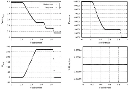
Figure 10.1 Density (top-left), pressure (top-right), average velocity (bottom-left) and void fraction (bottom-right) for the Sod shock tube . . . 74 Figure 10.2 Void fraction (left) and pressure (right) for the moving contact discontinuity 75 Figure 10.3 Comparison of the void fraction profiles with and without THINC

recon-struction . . . 76 Figure 10.4 Void fraction for the Faucet problem at t = 0.1s, 0.3s and 0.5s with exact

solution at 0.5s . . . 77 Figure 10.5 Void fraction for the Faucet problem using 500, 1000 and 10000 cells at 0.5s 77 Figure 10.6 Enlarged view of void fraction for the Faucet problem using 500, 1000 and

10000 cells at 0.5s . . . 78 Figure 10.7 Void fraction (top-left), pressure (top-right), average velocity (bottom-left)

(12)

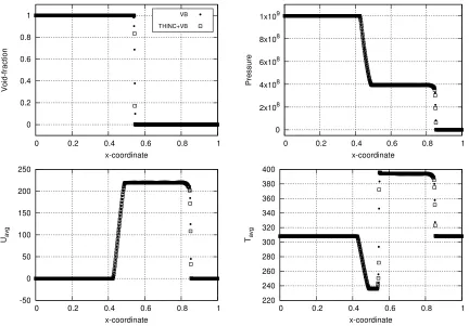
Figure 10.8 Comparison of the void fraction profiles for the air-water shock tube with and without THINC reconstruction . . . 80 Figure 10.9 Void fraction (top-left), pressure (top-right), average velocity (bottom-left)

and temperature (bottom-right) for the water-air shocktube . . . 81 Figure 10.10 Zoomed view of the void fraction (left) and pressure (right) for the water-air

shocktube showing material interface and shock capturing respectively. . . . 81 Figure 10.11 Void fraction (top-left), pressure (top-right), average velocity (bottom-left)

and temperature (bottom-right) for the high pressure ratio water-air shock tube . . . 83 Figure 10.12 Comparison of the void fraction profiles for the water-air shock tube with

and without THINC reconstruction . . . 83 Figure 10.13 Pressure profiles showing grid-convergence for the high pressure ratio

water-air shock tube (left); and an enlarged view near the shock(right) . . . 84 Figure 10.14 Pressure and numerical Schlieren contours for the shock/water-column

in-teraction at t= 6.25 µs (top), t= 10µs (middle), andt= 18.75 µs (bottom) 86 Figure 10.15 Numerical Schlieren (top-half) and volume fraction (bottom-half) contours

for the shock/water-column interaction using THINC (left) and without using THINC reconstruction (right) at flow-timest= 50µs,t= 100µs, and t= 200µs . . . 87 Figure 10.16 Pressure and numerical Schlieren contours for the shock/bubble interaction

att= 1.25 µs, 2.5µs, 3.75 µs, 4.75 µs, and 6 µs (top to bottom) . . . 90 Figure 10.17 Pressure and numerical Schlieren contours for the shock/bubble interaction

at t = 1.25 µs, 2.5 µs, 3.75 µs, 4.75 µs, and 6 µs (top to bottom) using unstructured mesh . . . 91 Figure 10.18 Top: Numerical Schlieren at 2.4 µs: Water-shock transmitted into bubble.

Bottom: Numerical Schlieren 3.825 µs: Bubble collapses onto itself and the air-shock is transmitted out. Left: Structured mesh. Right: Unstructured mesh. . . 92 Figure 10.19 Numerical Schlieren (top-half) and volume-fraction (bottom-half) contours

for the shock-He cylinder interaction test att= 80µs, 240µs, 420µs, 680µs, and 980 µs. THINC (left-column) compared to experiments from Haas and Sturtevant (1987) [25] (right-column) . . . 94 Figure 10.20 Numerical Schlieren (top-half) and volume-fraction (bottom-half) contours

for the shock-R22 cylinder interaction test (left-column) att= 50µs, 250µs, 420µs, 1020µs compared to experiments from Haas and Sturtevant (1987) [25] (right-column) . . . 96 Figure 10.21 Numerical Schlieren (left-half) and volume-fraction (right-half) contours for

(13)

Figure 10.27 Velocity profiles compared with BoilEulerFOAM results . . . 103

Figure 10.28 Contours of SA working variable ˜ν1 . . . 104

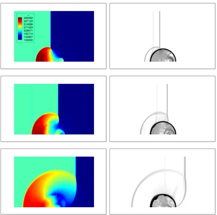
Figure 10.29 Water volume-fraction contours for the transverse jet injection problem at att= 0.5 ms (top-left), 1 ms (top-right), 1.5 ms (center-left), 2 ms (center-right), 3 ms (bottom-left), and 8.5 ms (bottom-right) . . . 106

Figure 10.30 Density contours for the transverse jet injection problem superimposed with streamlines at pseudo steady-state . . . 107

Figure 10.31 Pseudo steady-state for the transverse jet injection problem; Mach number (left) and SA turbulence working variable with volume-fraction contour lines (right) . . . 107

Figure D.1 Structured mesh used for shock-bubble interaction problem . . . 129

Figure D.2 Unstructured mesh used for shock-bubble interaction problem . . . 130

Figure D.3 Unstructured mesh used for underwater detonation problem . . . 130

(14)

Chapter 1

Introduction

(15)

bubble-coalescence or breakup and condensation. In situations where average-states of the multiphase flow are of interest and resolution of interfaces is not important, the EFM is used.

The EFM is derived from individual continuum equations for each phase, called the local instant formulation, and then applying an averaging procedure [31]. Assuming velocity and thermal non-equilibrium but pressure equilibrium, leads to the 6-equation Wallis model [86] of two-fluid flows. Solving the 6-equation model is a challenging problem. Legacy multiphase codes use pressure-based methods and resort to numerical diffusion and Picard-type iterations to make the system stable. Many of these methods resort to adding dissipation by the means of staggered grids and other techniques to obtain stable numerical results [69, 71]. These methods are usually termed as pressure-based algorithms since the working variable is pressure. They fall under the general class of operator-splitting type of methods. Pressure-based methods are better conditioned for lowM aflows, since at these speeds, the density is practically constant, and small errors in density (due to spatial or temporal discretizations) translate to large errors in pressure. Also, The pressure-based methods eliminate the speed of sound by reformulating the continuity and momentum equations by assuming that the velocity field is solenoidal (∇ ·v = 0). This results in a CFL criterion based solely on the flow velocity, independent of the acoustic speed, and larger time-step sizes leading to faster convergence. These pressure-based algorithms have been used successfully to obtain very accurate results for low speed flows, both for single-phase flows [8,62] and two-phase flows [24,71]. However, since these methods use operator-splitting to decouple the momentum and energy equations, compressibility can not be rigorously treated. The incompressibility assumption is deeply ingrained in their formulation. These algorithms result in significant inaccuracies and instabilities when high-temperature phenomena such as boiling and other problems involving large density gradients need to be simulated.

An alternative, potentially more promising approach is to use the density-based (fully com-pressible) method for multiphase flows. However, there are a number of issues in solving the 6-equation model by use of a density-based method:

• Extremely low-speed flows (M a <0.001): Many multiphase flows in engineering applica-tions are very low Mach number flows. This is known to cause difficulty in convergence. Also, the time-steps satisfying stability conditions (acoustic CFL) are too small to be feasible. The Riemann fluxes used in conventional compressible density-based methods tend to be highly diffusive in theM a <0.01 flow regime.

• High contribution of source terms: Interfacial force terms such as drag, interphasic mass transfer, etc. have such large contribution to the residual vector that the stable time-steps are further lowered.

(16)

has two possibly complex eigenvalues in its standard form. Naive discretizations employing density-based (hyperbolic) methods fail due to this.

• Non-conservative spatial and temporal derivatives: If discretized incorrectly, these can prevent preservation of stationary contact discontinuities.

One way to resolve low M a convergence issue is to solve the two-fluid system in a fully-implicit way using a primitive variable transformation matrix. Nourgaliev and co-workers [57,67] have used a [p,v, T]-formulation to solve near-incompressible flows using fully compressible density-based solver. Using pressure as a primitive variable makes the implicit density-based system better conditioned. Treating the source terms due to interfacial forces and phase-changes implicitly also relaxes the time-step restrictions, leading to faster convergence times.

(17)

In an attempt to obviate the need of the complete eigenstructure, it is desirable to use a numerical flux function such as AUSM. However, the regular AUSM+-up flux suffers from negative pressures in the regions of high pressure shocks interacting with material interfaces. This has been shown by studies by Kitamura [34, 35]. The solution proposed by Chang and Liou [11] was to use an exact Riemann solver, as mentioned before. The exact Riemann solver requires large number of Newton iterations to get a correct middle-zone pressure p∗ in the regions of question, thus making it expensive. A flux scheme which is robust enough in these regions, yet not invoking an iterative procedure, is presented here. This involves a modification to the baseline AUSM+-up fluxes via a volume-fraction coupling term in the mass-flux, resulting in what is called the AUSM+-upf flux in this work. This is similar to the Lax-Friedrich type dissipation employed by Houim and Oran [29] in the context of granular flows. Further, viscous flows, which are common in practical multiphase scenarios, are also solved using this method. The Spalart-Allmaras turbulence model is used to close the Favre-averaged two-fluid system. Eddy-viscosity of the continuous phase only is considered, with the assumption that the eddy-viscosity of the dispersed phase is linearly dependent on that of the continuous phase. The objective of this work thus, is to develop a density-based method for the solution of the turbulent two-fluid single pressure model which can be used as a baseline to develop a solver for more complex multiphase scenarios. The target applications for this work involve flows that require interphasic coupling using the drag force. Interphasic mass transfer effects are neglected.

Another approach to close the incomplete EFM two-fluid system is by including an addi-tional equation for volume fraction. This addiaddi-tional equation leads to a 7-equation two-pressure system, which is hyperbolic [4]. The Baer-Nunziato model has been extensively used for model-ing granular two-phase flow. This model was used by Saurel et al. [72–74], where the importance of a well-balanced discretization of non-conservative products was highlighted. It was established from this work that well-balancedness is necessary in preservation of a contact wave in a uni-form pressure and velocity field. This work used an infinite pressure and velocity relaxation as special cases to a more general 7-equation model, which allows non-equilibrium of phasic pressures, velocities and internal energies. In a following work [2], this assumption was relaxed and true non-equilibrium two-phase flows were solved using the discrete equation method.

(18)

applications is the presence of both high and very low Mach number flows in the same domain. It is obvious at this point that simulating truly compressible two-phase flows in a robust and efficient manner is a staggering task. It is after realizing this, that a decision was made, to deal with these complexities one-by-one. This kind of “bottom-up” approach allows the detailed study of each of the mathematical and numerical nuances of the complete two-phase system, which then can get addressed individually; rather than all at once, which would be a formidable task. With these challenges in mind, the need for a reliable two-phase flow solver was found to be the requisite primary task. Reliability comprises of robustness and accuracy. Thus, the primary objective of this work is to develop a robust and accurate two-phase flow method. Gen-erality in terms of equations of state is desired. Computational efficiency is another practical consideration. The presented two-phase solution method has been designed with these goals in mind. As work progressed, the method was found to be effective for sharp-interface/shock interaction problems as well. To further enhance this capability, the hyperbolic-tangent inter-face sharpening (THINC) method was implemented. The resulting algorithm is able to handle separated as well as dispersed/mixed flow two-phase problems.

(19)

Chapter 2

A background of two-phase modeling

Over the past few decades, a large number of ways to model interfaces in multiphase flows have been developed. Each of these methods was developed for specific applications and thus made use of different naming conventions. Due to this, there is a need to clarify certain definitions to be used in this thesis before beginning to describe two-phase models.

First and fore-most, the meaning of the words two-phase, two-fluid and multi-material flows needs to be mentioned:

• Two-phase: Flows involving two phases of the same fluid.

• Two-fluid: Flows involving two entirely different fluids.

• Multi-material: Flows involving multiple substances with potentially very different mate-rial properties.

(20)

2.1

Some basic definitions

2.1.1 Relative velocity

The relative velocity between two phases is defined as

Ur=Ud−Uc, (2.1)

where the subscriptsc and drepresent continuous and dispersed phases respectively.

2.1.2 Volume fraction

The volume fractionα of a fluid is its volume divided by the total volume of all fluids present:

αk=

Vk P

iVi

. (2.2)

2.1.3 Numerical Schlieren function

Schlieren imaging is widely used in experimental fluid dynamics to visualize shocked flow. In single phase computations, Schlieren images can be reproduced by the density gradient contours. For two-phase flows however, some scaling is required to be able to visualize shocks, rarefactions and contact waves in both fluids. Here, the numerical Schlieren function used is,

Sn= log (|∇ρm|+1), (2.3)

whereρm=α1ρ1+α2ρ2 is the mixture density.

A brief overview of the available multiphase models is justified at this point. This will help the reader get an idea about the peculiarities of each method, and also understand the specific model used in this work. Note that this is by no means a comprehensive literature review of all the multiphase methods.

As previously mentioned, multiphase models can be broadly classified into two types: the interface tracking type, and the diffuse interface type.

2.2

Interface tracking methods

(21)

in one fluid, and ‘1’ in the other, with intermediate values in cells which contain free surfaces. The level-set method [59] advects a distance-function, which is the distance from an interface; i.e. as the value of this function crosses zero, the two-phase interface is crossed. The front-tracking method [83] involves explicit reconstruction of the interface topology using a surface mesh, and then tracking this interface mesh. In all these methods, although there is sharp interface tracking, one must note that a small thickness of the order of the mesh size is allowed for transition of one fluid to the other. Another method of the Lagrangian type, the arbitrary Lagrangian Eulerian (ALE) method [50, 61], has recently been used for two-phase and multi-material flow problems. In this method, the mesh is itself moved with the interface, resulting in sharp interface tracking.

These type of interface tracking methods are extremely accurate in resolving material in-terfaces. This level of accuracy is justified when surface dynamics such as effect of surfactants on surface tension, bubble-dynamics etc. are the subject of study. However, this high accuracy comes with added implementation complexity and computation costs. Topology changes such as bubble collapse, coalescence and droplet breakup are extremely challenging to handle in level-set, front-tracking and ALE methods. Moreover, in many engineering applications, the exact surface resolution is not important, and only average quantities, such as phasic velocities, temperatures, heat transfer and of interest. In such situations, usually there are hundreds of thousands of bubbles in the continuous phase. Using an interface tracking technique in this situ-ation would be extremely expensive. These are the type of situsitu-ations where the diffuse interface type of models are useful.

2.3

Diffuse interface models

(22)

2.3.1 Homogeneous two-phase model

One of the earliest Eulerian two-phase models was the mixture model (cf. [86]) also known as the homogeneous two-phase model, for reasons of thermodynamic equilibrium between the two phases at every point in space. This means that the velocity, pressure and internal energies of the two phases are assumed to equilibriate instantaneously. The governing equations consist ofn−1 mass/volume fraction, one total mass conservation, one mixture momentum conservation and one total energy conservation equations; with the compatibility relation that the summation of mass/volume fractions is one. In specific cases, there can be multiple energy equations, pertaining to thenfluids or non-equilibrium between the different thermal modes, depending on the problem being solved. The assumptions of velocity and specific internal energy equilibrium between two phases is only valid for certain kinds of flows, but not for others. Bubbly flows in reactors have different fluid velocities and internal energies; thus rendering these assumptions inaccurate for such flows.

2.3.2 Drift-flux model

Another two-phase model which somewhat relaxes the equal velocity assumption is the drift-flux model. The drift-drift-flux model [89] has an additional transport equation for the relative velocity between the two phases. However, the formulation of the drift-flux model inherently assumes that the relative velocity is small compared to the continuous phase velocity. If the drift-flux velocity becomes very high, the drift-flux model can be proven to be non-hyperbolic. The assumption of small relative velocities does not hold true for many engineering scenarios. Besides, the internal energies of the two fluids are assumed to be in equilibrium for the drift-flux model too. Thus, this model is unsuitable for the target applications in this work.

2.3.3 Single pressure non-homogeneous two-phase flow model

(23)

instantaneous pressure relaxation assumption, especially at very high speeds. Nevertheless, this model is an appropriate candidate for the applications targeted here.

2.3.4 Two pressure non-homogeneous two-phase flow model

Another two-phase model, which does not assume pressure equilibrium in the two phases is the two-pressureseven-equation model. The two-pressure model was developed by Baer and Nunzi-ato [4] originally for particle/granular flows, and followed up by Kapila et al. [6, 32]. Due to the additional unknown (second pressure), another equation is necessary for closure. A transport equation for the volume fraction is appended to the original six transport equations. This model can be proven to be strictly hyperbolic, and therefore has gained significant attention in recent years. A pressure relaxation needs to be performed to preserve interface-capturing capabilities of this model. This has brought up the question of why the separate pressures (and thus the additional transport equation for volume fraction) are required in the first place. Nevertheless, this model is also a prospective candidate for this work.

(24)

Chapter 3

Governing Equations

As described in the previous chapter, the fluid model is a diffuse interface type of two-phase model. This means that the interpenetrating continua assumption is used to formulate the governing equations. The interpenetrating continua approach assumes that at each point in the fluid domain, both the phases are present. The proportions (volume fractions) may vary widely, but nevertheless, each phase is present everywhere, in however small a quantity. For example, in a “pure” liquid region of the flow, it is assumed that the vapor phase is present in a very tiny quantity. It will be seen later that a very small value of volume fraction (10−7 to 10−5_{) is used to define such a “near single-phase” zone.}

3.1

The inviscid two-fluid model

The two-fluid model uses the interpenetrating continua approach to model two-phase flows. This model requires an averaging procedure to filter-out the local instantaneous fluctuations very similar to the Reynolds’ averaging in turbulence. As mentioned earlier, interphasic mass-transfer terms have not been considered in this work. The resulting inviscid two-fluid model given by Ishii [31] and concisely by Staedtke [77], using k as the index for the two fluids, is as follows:

∂Uk

∂t + ∂Fkj

∂xj

(25)

where,

Uk= 

 

αkρk

αkρkuki

αkρkEk 



 (3.2)

Fkj =



 

αkρkukj

αkρkukiukj

αkρkukjHk

  +    0 αkpδij

0





 (3.3)

Pint_k =

   0 pint k ∂αk ∂xi

−pint_k ∂αk

∂t 



 k= 1,2. (3.4)

Sk represent source terms, for example due to phase transitions and body forces.

In 1D, the system (3.1) has 11 unknowns (αk, ρk, uk, Ek, pintk , pwithk= 1,2) and a total of

9 equations with 6 PDEs, 2 equations of state (EoS) and the constraint on volume fractions,

2

X

k=1

αk= 1. (3.5)

These equations constitute the Wallis two-fluid model or the 6-equation single-pressure model of two-phase flows. The EoS required to close this system are given in the next section. Another condition that the interfacial pressures should cancel each other if no other stresses such as surface tension are considered at the interface gives,

pint₁ =pint₂ ≡pint. (3.6)

pint is explicitly given as a function of the other unknowns. Here, we use the relation given by Stuhmiller [80],

pint=p−σ α1α2ρ1ρ2 α1ρ2+α2ρ1

u2_r (3.7)

whereur =|u2−u1|. This form of the interface pressure term was used and validated first by

(26)

the above interface pressure be kept within limits using:

pint = min(pint,0.01p). (3.8)

This provides the additional 3 equations and the system of equations is closed. The effect of addition of the interface pressure term has been analyzed in detail by Chang et al. [12]. They show that there is a limiting value of σ above which the system (3.1) is hyperbolic. Here, a value of σ= 2 is used for all the problems.

3.2

Equations of state

The stiffened-gas equations of state (SG-EoS) are used for each fluid in this work. Using the SG-EoS, the pressure, temperature and speed of sound are given respectively as:

ρEk =

p+Pck

γk−1

+ρu 2

k

2 +Pck (3.9)

Tk =

γk

γk−1

(p+Pck)

ρkCpk

(3.10)

ak = s

γk

p+Pck

ρk

. (3.11)

The following properties are used for the ideal gas phase and the liquid phase:

Table 3.1: Properties in SG-EOS

Property Gas Liquid

γ 1.4 2.8

Pc[P a] 0.0 8.5×108

Cp[J/(kg·K)] 1004.5 4186.0

3.3

Turbulent two-fluid model

(27)

of the simpler models is the Spalart-Allmaras model, which uses the isotropic turbulence as-sumption to model the Reynolds stresses via the SA working variable ˜ν, which is a function of the eddy-viscosity. The modified Spalart-Allmaras model [3] is used here. In this work, only the SA working variable for the continuous phase is solved for, and the dispersed phase turbulence is modeled using a response coefficient.

In turbulence literature, the averaged quantities are denoted by an overbar (·). However, for simplicity of notation, this overbar is skipped in the following, with the understanding that, if the RANS equations are being solved, the flow quantities being referred to, are averaged flow quantities. Considering this, the turbulent two-fluid equations are given as:

∂Uk

∂t + ∂Fkj

∂xj

= ∂Gkj ∂xj

+Pint_k +Sk (3.12)

where,

Uk=      

αkρk

αkρkuki

αkρkEk

α1ρ1ν˜1

      (3.13)

Fkj =

     

αkρkukj

αkρkukiukj

αkρkukjHk

α1ρ1u1jν1˜

      +       0 αkpδij

0 0      

, Pint_k =

      0 pint k ∂αk ∂xi

−pint_k ∂αk

∂t 0       (3.14)

Gkj =

      0 αkτkTij

αkuklτ

T

klj +αkqkj

α1_σ1µ1(1 +ψ)∂_∂xν˜1_j

      (3.15) S=       0 Mki

ukjMkj

Sν˜1      

k= 1,2. (3.16)

Mk are interface forces such as drag and virtual mass. and body forces such as gravity. S˜ν

(28)

given as,

τ_ijT = (µ+µT)

∂ui

∂xj

+∂uj ∂xi −2 3 ∂ul ∂xl δij

, qj =Cp

µ P r +

µT

P rT

∂T ∂xj

, (3.17)

where,

µT = 





ρνf˜ v1 if ˜ν ≥0

0 otherwise.

(3.18)

where the fluid-index khas been dropped for convenience. Note that the fluid properties (viz. µ,P r ,Cp) are fluid specific. These properties are specified for each phase and kept constant in

the scope of this work. As mentioned before, turbulence in the dispersed phase is not separately modeled, but accounted for by a response coefficient. Physically this means that the eddy-viscosity of the dispersed phase is a function of the continuous phase eddy-eddy-viscosity. In the scope of this work, the response coefficient is set to be 1, i.e. the eddy-viscosities in the two fluids are equal.

The modified Spalart-Allmaras model [3] is used for turbulence closure of the continuous phase. The Favre-averaging for compressible flows are described in detail by Luo and coworkers [13, 47] and references cited therein. Details are repeated here for completeness.

The Favre-averaged conservation law for the SA working-variable is given by,

∂α1ρ1ν˜1 ∂t +

∂α1ρ1u1jν˜1

∂xj = ∂ ∂xj α1 1

σµ1(1 +ψ) ∂ν˜1 ∂xj

+Sν˜1, (3.19)

and the source term is,

S˜ν1 =α1 cb1Sµ1ψ˜ +

1

σcb2ρ1∇ν˜· ∇ν˜−cw1ρ1fw

ν1ψ d

2!

. (3.20)

This version of the SA model was proposed by Allmaras et al. [3] to make the original model more robust. The first modification to remove the effects of negative ˜ν is by the usage of the following parameter in the diffusive term:

ψ=







0.05ln(1 +e20χ) ifχ≤10

χ otherwise,

(29)

where,

χ= ρν˜

µ . (3.22)

The second modification aims at eliminating the possibility of ˜Sin the production term reaching zero or negative values:

˜ S =







S+ ˆS if ˆS≥ −cv2S

S+ S(c2v2S+cv3Sˆ)

(cv3−2cv2)S−Sˆ otherwise,

(3.23)

where,

S=

√

−→_ω _{· −}→_{ω ,} _S_ˆ₌ νψ

k_T2d2fv2, fv1= ψ3 ψ3₊_c3

v1

, fv2= 1− ψ 1 +ψfv1

. (3.24)

Here−→ω denotes the vorticity vector∇ ×uanddis the distance to the nearest wall at a specific location in the flow domain. The constants used in the model are,

σ= 2

3, cb1 = 0.1355, cb2 = 0.622, kT = 0.41, cw1 = cb1 k2

T

+1 +cb2

σ , (3.25)

cw2= 0.3, cw3= 2, cv1= 7.1, cv2 = 0.7, cv3= 0.9, P rT = 0.9. (3.26)

The working-variable ˜ν generally is orders of magnitude larger than the other state variables in the fully developed turbulent flow regime. Thus, the SA-equation is scaled with√Refor ease of convergence. Further details about the Spalart-Allmaras model can be found in the references. The interface momentum transfer termsMK are now described.

3.4

Drag force model

The drag-force interfacial momentum transfer term is modeled as,

M1 =−M2 = 3 4Cd

ρ2α1 db

|Ur|Ur, (3.27)

where the relative velocity is,

Ur=U2−U1. (3.28)

(30)

as a constantCd= 2.0. The bubble/droplet diameter is denoted bydb. A value ofdb= 1.0mm

is used for the tests in this article.

3.5

Virtual mass force model

The presence of virtual mass force improves the stability of the numerical scheme in regions of high accelerations, for flows with a high density ratio [37]. This force is modeled as,

Mvm₁ =−Mvm₂ =Cvmρ1α1α2

D2(u2) Dt −

D1(u1) Dt

, (3.29)

with the same notation for the subscripts as the drag force. The phasic material/substantial derivatives of the quantity ψare given as,

Dkψ

Dt = ∂ψ

∂t +uk· ∇ψ. (3.30)

These substantial derivatives are treated part-implicitly, such that they improve the condition number of the system. In other words, the positive contribution to the diagonal entries of the system matrix are treated implicitly, and the rest, explicitly. The virtual mass force is used only in the viscous problems in this work. The virtual mass coefficient is set as Cvm= 0.5.

3.6

Non-dimensionalization of the RANS-SA two-fluid system

Non-dimensionalization is a common practice in solving the compressible turbulent flow equa-tions. One benefit of using non-dimensionalized forms are that dimensionless quantities such as the Reynolds number (Re), the Mach number (M), and the Prandtl number (P r) appear in the equations directly and thus can be varied independently. Another benefit is that the flow variables are normalized, i.e. their values fall within prescribed limits, which could make it easier to work with them. A disadvantage of working with non-dimensionalized forms of the equations is that the physical properties such as dynamic viscosity (µ), thermal conductivity (k), and specific heat (cp) do not appear in the equations directly, but via the dimensionless

quantities. This forces the user to work with dimensionless quantities, even if the values of the physical variables are readily available. Here, the non-dimensionalized forms are used, so that the important dimensionless quantities can be directly altered for testing purposes.

(31)

density and reference speed of sound used for non-dimensionalization. The reference quantities used in this work are listed in Table 3.2.

Table 3.2: Reference quantities used for non-dimensionalization

Variable Reference

Length,Lref 1

Velocity,Vref Freestream speed of sounda∞

Pressure,Pref Problem dependent reference pressure

Temperature, Tref Freestream temperatureT∞

Viscosity, µref Freestream viscosityµ∞

The reference density and time, which are derived reference quantities can now be obtained as,

ρref =

pref

a2

∞

, tref =

Lref

a∞

. (3.31)

The volume fraction αk is dimensionless to begin with, and does not require any further

non-dimensionalization. Using the above reference quantities, the non-dimensionalized variables can then be written as follows:

L∗= L Lref

, u∗_k_j = ukj a∞

, p∗ = p pref

, ρ∗_k = ρk ρref

,

C_p∗

k =

Cpk

a2

∞T∞

, E_k∗ = Ek a2

∞

, ν˜_k∗ = ν˜k µ∞/ρref

. (3.32)

Using these definitions, the non-dimensional phasic continuity, momentum and energy equations can be written as follows:

∂

∂t(αkρk) + ∂ ∂xj

(αkρkukj) = 0 (3.33)

∂

∂t(αkρkuki) +

∂ ∂xj

(αkρkukiukj) +αk

∂p ∂xi

= Mref Reref

∂αkτijT

∂xj

+ Lref ρrefa2∞

(M_k†

i) (3.34)

∂

∂t(αkρkEk) + ∂ ∂xj

(αkρkHkukj) =−p

∂αk

∂t

+ Mref Reref

∂ ∂xj

αkuklτ

T

lj +αkCp

µ P r +

µT

P rT

∂T ∂xj

+ Lref ρrefa2∞

(ukjM

†

kj), (3.35)

(32)

·† _{are non-dimensionalized according to Eq. (3.32). The terms represented as} _·† _{will be}

non-dimensionalized separately.Mref and Reref are the reference Mach and Reynolds numbers,

Mref =

uref

a∞

, Reref =

ρrefurefLref

µ∞

. (3.36)

The reference velocity uref used in the above definitions in Eq. (3.36) is arbitrary, since Mref

andReref occur in the governing equations only as a ratio. As long as the same velocity is used

in both the definitions, the non-dimensionalization is consistent with the dimensional equations. The Spalart-Allmaras equation also needs to be non-dimensionalized consistently with the other equations. The dimensionless form of the SA equation, using the definition of ˜ν∗ from Eq. (3.32) is,

∂α1ρ1ν˜1 ∂t +

∂α1ρ1u1jν˜1

∂xj

= Mref Reref ∂ ∂xj α1 1

σµ1(1 +ψ) ∂ν˜1 ∂xj

+

Mref

Reref

α1 cb1

Reref

Mref

S+ ˆS

µ1ψ+ 1

σcb2ρ1∇ν˜· ∇ν˜−cw1ρ1fw

ν1ψ d

2!

, (3.37)

where again the ·∗’s have been dropped. As mentioned previously, the SA equation is scaled withp

Reref. Considering the definition ˜ν 0

= ˜ν/p

Reref, the final form of the SA equation can

be derived to be,

∂α1ρ1ν˜

0

1 ∂t +

∂α1ρ1u1jν˜

0

1 ∂xj

= Mref Reref

∂ ∂xj

α1 1

σµ1(1 +ψ) ∂ν˜1

0

∂xj !

+

Mref

Re3_ref/2

α1 cb1

Reref

Mref

S+ ˆS

µ1ψ+ Reref

σ cb2ρ1∇ν˜

0

· ∇ν˜0 −cw1ρ1fw

ν1ψ d

2!

. (3.38)

Detailed procedure to obtain this final non-dimensionalized form are given in Appendix A. The inviscid part of the non-dimensionalized governing equations are the same as the dimensional form of the equations. The dimensionalization changes the viscous terms only. These non-dimensionalized equations are discretized in the present work.

(33)

Chapter 4

Eigenvalues and the acoustic speed

The eigenvalues and eigenvectors (collectively called the eigensystem) of a system of partial differential equations determine the mathematical nature of that system. The mathematical nature determines the appropriate algorithm used to obtain the numerical solution of this system. The eigenvalues also play a key role in spatial-discretization for hyperbolic systems. The importance of an eigenvalue analysis of a system before designing a numerical method for it, is thus evident.

To this end, the eigenvalue analysis of the two-fluid model has been performed and the results are noted here. Only the inviscid part of the one-dimensional governing equations is analyzed to judge the mathematical nature of the system. It is known that the viscous terms make the system parabolic. However, the discretization of the inviscid (convective) flux terms depend heavily on the eigenvalues of the inviscid system, because of which this system is analyzed. Previous work by St¨adtke [77] and Chang et al. [12] are the primary references for this analysis. Analyzing eigenvalues becomes easier if certain “primitive” variables are considered and then a transformation to these primitive variables is carried out. Quite a few choices for this are possible:

• [α1, p, u1, u2, s1, s2] as [77], where sk is the k-phase entropy; • [α1, p, u1, u2, ρ1, ρ2] as [12], etc.

The choice of primitive variables made here is: [T1, u1, T2, u2, p, α1]. This set of primitive variables is also used in the implicit time-stepping scheme [57, 67] to better condition low Mach number flow problems. The same primitive variables are used in this section to avoid any confusion.

(34)

In addition to these 4 common eigenvalues, the full two-fluid system has 2 other eigenvalues: (u1, u2). Thus, analyzing the four-equation isothermal system is sufficient.

4.1

Eigenvalue analysis

As mentioned above, the eigenvalue analysis becomes easier if primitive variables are considered. For this purpose, the Jacobian of transformation is first derived. The conservative variables and the primitive variables for the isothermal two-fluid system are:

U=      

α1ρ1 α1ρ1u1

α2ρ2 α2ρ2u2

      V=       α1 p u1 u2       . (4.1)

The transformation matrix is,

∂U ∂V =

     

ρ1 α1(ρ1)p 0 0

ρ1u1 α1(ρ1)pu1 α1ρ1 0 −ρ2 α2(ρ2)p 0 0 −ρ2u2 α2(ρ2)pu2 0 α2ρ2

      , (4.2)

where (ρk)p≡ ∂ρ_∂pk, and depends on the equation of state used for fluid-k. Using these definitions,

the two-fluid equations can be written as,

∂U ∂V ∂V ∂t + ∂F ∂V ∂V ∂x =Cx

∂V

∂x, (4.3)

where,

Cx =      

0 0 0 0

pint ₀ ₀ ₀

0 0 0 0

−pint 0 0 0

      . (4.4)

Following some simple algebraic manipulations, the standard form can be obtained:

∂V ∂t + ∂U ∂V −1 ∂F ∂V −Cx

∂V

(35)

The eigenvalues of the system matrix A≡ ∂U ∂V −1 ∂F ∂V−Cx

(4.6) = ∂U ∂V −1      

ρ1u1 α1u1(ρ1)p α1ρ1 0 ρ1u2₁+p−pint α1u2₁(ρ1)p+α1 2α1ρ1u1 0

ρ2u2 α2u2(ρ2)p 0 α2ρ2

−(ρ2u22+p−pint) α2u22(ρ2)p+α2 0 2α2ρ2u2

      . (4.7)

are to be analyzed.

A few important observations can be made at this point. Wallis’ two-fluid model [86] assumes p=pint. It can be shown [77] that Wallis’ model has a pair of complex conjugate eigenvalues, thus making it non-hyperbolic. Several correction methods have been proposed, via regulariza-tion [16] or by corrective terms in the model equaregulariza-tions [7, 80]. Significant research effort has been based on the addition of hyperbolizing terms to the model equations [11, 54], the reason being that these models can be proven to have all real eigenvalues once these corrective terms are added. The “interface pressure” pint is one such corrective term widely used in literature. Chang et al. [12, 43] prove that above certain values ofσ (Eq. (3.7)), the two-fluid model is hy-perbolic. Cortes et al. [15] prove the same using perturbation methods, clearly stating that this interface pressure term is necessary for the two-fluid model to be hyperbolic. However, even though hyperbolicity can be proven for this model, explicit expressions for eigenvalues (and eigenvectors) cannot be derived. Eigenvalues dictate the acoustic characteristics of a hyperbolic system, and it is difficult to design a stable numerical scheme without the knowledge of at least the spectral radius (sum of acoustic speed and fluid velocity). The question then is: what is the acoustic speed (or speed of sound) of this system? Unfortunately, one is left with nothing but guesses as to what constitutes the speed of sound in the two-fluid system. Fortunately, there are a few educated estimates that one can use for this purpose. The next section discusses this in further detail.

4.2

Speed of sound

(36)

Wallis [86]. Wallis derived acoustic speeds for various systems of two-phase flow equations. He derived the acoustic speed for the “stratified” type of two-phase flow. A list of possible choices is included here, for the sake of completeness:

1. Wallis’ stratified flow [86]: _a12

c =

ρ1ρ2 α1ρ2+α2ρ1

α1 ρ1a21

+ α2 ρ2a22

,

2. Toumi [81]: a2_c = ρ(α1ρ2+α2ρ1) ρ1ρ2

∂p ∂ρ

3. Liou [43]: a2_c= a21a22(ρ1+ρ2) ρ1a2₂+ρ2a2₁

4. Averaged: ac= a1+₂a2

5. Maximum:ac= max(a1, a2)

Wallis’ speed of sound definition has been used by Chang and coworkers [11]. This seems to be the best choice in this regard. However, it must be noted here that this choice assumes that the relative velocity is zero. Although this is indeed the case for many pipe-flow applications, it is not the case for high-speed shocked two-fluid flows. This is an important point of consideration, which will be the basis of the modifications to the AUSM+-up flux.

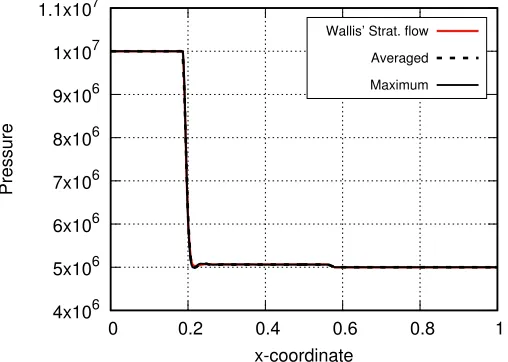
Nevertheless, a choice of an acoustic speed for usage in the flux function has to be made. A comparison was made using Wallis’, the average and the maximum speed of sound definitions in the two-fluid method proposed here. Pressure profiles of a water-air shocktube problem are shown in Figs. 4.1 and 4.2. For details about the problem setup, see Chapter 10.

4x106 5x106 6x106 7x106 8x106 9x106 1x107 1.1x107

0 0.2 0.4 0.6 0.8 1

Pressure

x-coordinate

Wallis’ Strat. flow

Averaged

Maximum

(37)

4x106 5x106 6x106 7x106 8x106 9x106 1x107 1.1x107

0.16 0.18 0.2 0.22 0.24 0.26

Pressure

x-coordinate

4.99x106 5x106 5.01x106 5.02x106 5.03x106 5.04x106 5.05x106 5.06x106 5.07x106

0.52 0.54 0.56 0.58 0.6

Pressure

x-coordinate

Figure 4.2: Pressure profiles for the water-air shock tube using the three speed of sound defi-nitions, zoomed in near the rarefaction wave (left) and the shock (right)

The pressure profiles obtained using Wallis’ definition, the average and the maximum speed of sound look similar in Fig. 4.1. On further inspection, some differences are noticed near the rarefaction wave. However, the most important differences are observed near the shock (c.f. the right graph in Fig. 4.2). Using the maximum speed of sound yields oscillatory results downstream of the shock. The shock-structure also seems to be step-like. Wallis’ speed of sound definition seems to produce the best shock-capturing for this example. For a higher pressure-ratio water-air shocktube, the average sound speed definition does not produce a stable numerical method. For these reasons, Wallis’ weighted harmonic speed of sound definition has been used in the flux definitions in this work.

4.3

Linear degenerate eigenvalues

(38)

non-SCD-preserving schemes. Liou and Steffen’s AUSM [41, 42, 45], Edwards’ LDFSS [19, 21] are some examples of S/MCD-preserving flux-vector splitting type of schemes. While discretizing the two-fluid model however, in addition of the discretization of flux terms, an additional factor requires to be taken into consideration: the non-conservative term. The importance of proper discretization of the non-conservative product has been emphasized by Abgrall et al. [1, 72], Par´es [66] and Toumi et al. [81, 82] The discretizations of the non-conservative term and the pressure flux together have to satisfy the well-balancedness or Abgrall’s criterion. This ensures capturing the correct physical behavior in situations of linear degenerate eigenvalues. In a later chapter (Ch. 5), the well-balancedness of the method used in this work is shown, indicating that linear-degenerate cases can be handled properly by the method.

4.4

Effect of the interface pressure term

It is natural to question the applicability of thenew two-fluid model resulting from the addition of the hyperbolizing term

pint =p−σ α1α2ρ1ρ2 α1ρ2+α2ρ1u

2

r,

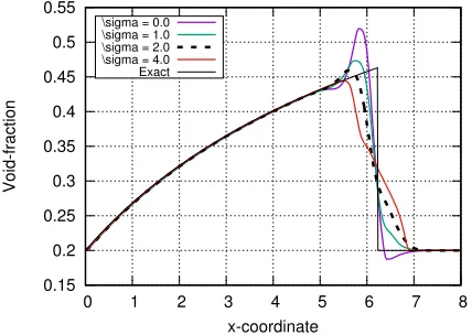
since this term changes the PDEs being solved. It has also been pointed out previously [22, 27] that this correction is insufficient to restore hyperbolicity in the originally non-hyperbolic model.

0.15 0.2 0.25 0.3 0.35 0.4 0.45 0.5 0.55

0 1 2 3 4 5 6 7 8

Void-fraction

x-coordinate

\sigma = 0.0 \sigma = 1.0 \sigma = 2.0 \sigma = 4.0 Exact

Figure 4.3: Effect of coefficientσ for the faucet problem

(39)

a mesh with 500 cells. Effect ofσ in the interface pressure is studied. The void-fraction profiles obtained usingσ= 0,1,2 and 4 are shown in Fig. 4.3. It is observed here that addition of the interface pressure term adds stability to the two-fluid model in the vicinity of large volume-fraction gradients, such as the void-wave in this problem. Oscillations near the void-wave are suppressed as the contribution of the interface-pressure term is increased. Without this term the volume-fraction would not be bound in the interval [0,1] at the material interface, on a finer mesh. However, it can also be seen that although this term provides stability, it is at the cost of a significant smearing of the interface. It is for this reason that the interface pressure parameterσ must not be set to an unreasonably high values. In the scope of this work, a value of σ= 2 is used for all the test problems.

With this preliminary analysis complete, the spatial discretization of each of the terms in the governing equations can now be discussed. As a summary, the following key factors need to be considered while discretizing the two-fluid model:

• The exact speed of sound is not known, and an appropriate choice of an expression for the speed of sound becomes critical;

• Possibility of linear degeneracy imposes additional constraints on the discretization of the pressure flux and non-conservative terms;

• If possible, interplay between the above two factors and interface pressure.

(40)

Chapter 5

Spatial discretization

Proper discretization of the two-fluid system Eq. (3.1) is critical if the numerical method is expected to be stable, robust and yield accurate results. This section describes the methods used to discretize the two-fluid system in detail. Spatial discretization is a very broad topic, and includes a myriad of sub-topics ranging from the numerical flux function used to solve the Riemann problem, to reconstruction and limiting with interface sharpening. A cell-centered finite volume method is used to discretize the equations, and second order accuracy is obtained using the least-squares reconstruction. Spurious oscillations arising from this reconstruction are eliminated using a vertex-based limiting for the flow-variables. The hyperbolic tangent interface sharpening (THINC) technique is used for the volume-fraction variable where sharp material interfaces are desired. The Riemann problem arising at each cell-face is solved using a modification of the AUSM+-up flux, henceforth called as the AUSM+-upf flux. A detailed description of the above methods is presented here.

This chapter is organized as follows. First, the non-conservative product terms in the mo-mentum equations and the finite volume integral form of the system are discussed, followed by details of the numerical flux function. The reconstruction to second order is discussed next. This section also describes the limiting process for the reconstructed gradients. This is followed by manual verification of the well-balancedness of the spatial discretization proposed in this work. Boundary conditions are described next.

5.1

The non-conservative pressure term

(41)

discretizations of non-conservative PDEs have been done, starting from Pares’ work [66], lead-ing to Roe-type [10] and Osher-type [18] schemes for these equations. A numerical method for the two-fluid equations specifically was also proposed based on this concept [51]. This collec-tion of work clearly states that well-balancedness is an essential property while designing a numerical method for solving non-conservative PDEs, to maintain global conservation. Abgrall, in one of his early works [1], also focuses on this property in the context of multi-species (or multi-component) equations.

The two-fluid momentum equation in its original form [31] is,

∂

∂t(αkρkuki) +

∂ ∂xj

(αkρkukiukj) +αk

∂p ∂xi

+δp∂αk ∂xi

= 0, (5.1)

whereδp is the interface pressure correction given in Eq. (3.7).

Consider a domain Ω with boundaries Γ. The pressure flux αk∇p and the other

non-conservative term δp∇αk on this domain can be simply written as,

Z Ω αk ∂p ∂xi

+δp∂αk ∂xi

dΩ.

Consider now, an element Ωe a part of the triangulation of Ω. Since these terms are

non-conservative, it is not clear how they should be discretized in this form. Thus, using integration-by-parts, the above term can be expanded on the element Ωe as,

Z Ωe αk ∂p ∂xi

+δp∂αk ∂xi

dΩ =

Z

Γe

αkpnidΓ− Z

Ωe

p∂αk ∂xi

dΩ +

Z

Ωe

δp∂αk ∂xi

dΩ (5.2)

=

Z

Γe

αkpnidΓ− Z

Ωe

(p−δp)∂αk ∂xi

dΩ, (5.3)

where ni is the i-component of the normal to the element boundary Γe, pointing outward of

Ωe. Since δp is a correction only, it is usually integrated like a source term.

Now, the first term is an integral over the cell-boundary Γe which uses the value of the

integrand (αkp) from the cell Ωe. This term takes into account the jump of the function at

each cell-boundary. The pressure for this term should be obtained by the Riemann solver used (AUSM+-upf in this case,pk,1/2) since otherwise it is not uniquely defined on the cell-boundary. On the other hand, the volume-fraction for this term is supposed to be reconstructed from the cell Ωe. Thus, on each cell-boundary, this term will have a different contribution to the cells

straddling the boundary only due to the volume-fractionαkin it. This term corresponds to the

pressure flux and will be discussed in the section describing the Riemann solver. The second term can be treated as a source term since it is an integral over the cell Ωe only. This clearly

(42)

one from each side of the face. This type of treatment ensures the well-balanced nature of the discretization. Thus, the “stratified-flow model” discretization of the non-conservative term [11] is obtained by applying integration-by-parts to the pressure term in the two-fluid model while writing it in the discrete form. This leads us to the momentum equation in the form shown in (3.1), where the first term in Eq. (5.2) has been absorbed into the flux term F, and the rest is denoted by the Pint interface-pressure term. A proof of the well-balancedness of this discretization will be given after the Riemann solver is discussed. Now that the discretization for the non-conservative terms is known, the discrete integral form of the inviscid (3.1) and turbulent (3.12) systems can be presented.

5.2

The integral form and finite volume method

The finite volume method is a well-known spatial discretization technique for solution of conser-vation laws. It is used to obtain a discrete solution for the conserved quantity by, first discretizing the physical domain into smaller sub-domains called finite or control volumes. Then algebraic balance equations are written for the conserved quantities in each of these control volumes. The “flux” of said quantities in and out of the control volumes is considered for this purpose. Discrete solutions to the conservation laws are computed using these algebraic balance equa-tions. For this, the solution polynomial over each of these computational cells is approximated by a constant cell-averaged value, and the algebraic balance equations are solved for these cell-averages over each cell. From the piecewise polynomial approximation of the solution, it becomes apparent that the solution is discontinuous at the boundaries of every computational cell, and because of this, the value of the solution is not uniquely defined at these boundaries. The solution value at the boundaries is required to compute the fluxes in the balance equations. This problem of having two piecewise constant but discontinuous states at the cell boundary is called a Riemann problem. There are various ways to solve the Riemann problem, and they depend on the conservation law being solved. These Riemann solvers give a single state de-pending on these left and right states, which is then used to write the fluxes in the balance equations. Once the algebraic balance equations are formed, they can be solved to obtain the discrete solution of the conservation law. Since there is error associated with this solution, it is also called the approximate or numerical solution. Details of the Riemann solver used in this work will be discussed in another section.

(43)

is hard to extend to unstructured grids. Another approach to higher order extension is the least-squares reconstruction, which is suitable for unstructured meshes too. The least-squares reconstruction attempts to reconstruct a piecewise linear solution polynomial from the piece-wise constant solution on each computational cell, using the piecepiece-wise constant solutions from the neighboring cells. Using such a reconstruction procedure yields a second-order spatial dis-cretization. This second-order finite volume method is used in this work. Further details about least-square reconstruction will be discussed in the relevant section.

The two-fluid system is discretized using the second-order finite volume method described above. Consider a domain Ω over which the two-fluid system is to be solved, and its triangu-lation Ωe ∈Ω. The boundaries of each mesh element Ωe are denoted by Γe. The finite volume

approximation is now applied to this discrete domain. On integrating over each elemente, and applying the divergence theorem on the flux terms, the semi-discrete system (balance equations) can be written as,

Z

Ωe

∂Uk

∂t dΩ +

Z

Γe

(Fk·n) dΓ− Z

Γe

(Gk·n) dΓ = Z

Ωe

Pint_k +Sk

dΩ. (5.4)

Here, the cells are denoted by Ωe, the cell-faces by Γe and nis the unit normal to Γe, pointing

outward of Ωe. The second and third terms on the left-hand side of Eq. (5.4) represent inviscid

and viscous fluxes across cell boundaries Γe respectively. As mentioned previously, a Riemann

solver is required to compute the inviscid fluxes on Γe. The Riemann solver used in this work

is discussed now, followed by the computation of the viscous fluxes.

It should be noted here that the system in Eq. (5.4) is not fully discretized, since the time-derivatives are still present. Discretization of the time derivative will be discussed in the next chapter.

5.3

The Riemann solver

(44)

For example, consider the followingdiagonalizable non-linear system and its linearization, ∂U

∂t +

∂F(U)

∂x = 0 (5.5)

∂U ∂t +A

∂U

∂x = 0 (5.6)

∂U ∂t +R

−1_ΛR∂U

∂x = 0, (5.7)

whereRis the matrix of right eigenvectors, which can be proven to be a matrix of transformation to thecharacteristic variables of the system:

R= ∂W

∂U, (5.8)

and Λ = diag[λi] is the diagonal matrix of eigenvalues of the system. Thus, the above system

can be simplified as,

∂W ∂t +Λ

∂W

∂x = 0, (5.9)

(45)

Broadly, the inviscid fluxes in the two-fluid model can be discretized using two types of methods as described by Kitamura et al. [34]:

1. AUSM-family standalone: The all-speed variant AUSM+-up developed by Liou [42] and extended to the stratified-flow two-fluid model in [43] is employed in this type. A single flux-function is used to computed the flux at the cell-interfaces. Other FVS-type schemes such as Edwards’ LDFSS [19], AUSMPW+ by Kim et al. [33], and Niu’s AUSMDV [53] can also be used instead of AUSM+-up, with the appropriate modifications in the scaling terms.

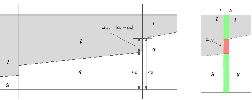
2. Hybrid AUSM+Riemann (Godunov) solver: Flux at the cell-interface is split into fluxes betweenlikephases (l-l, g-g) andunlikephases (l-g, g-l), wherelandgrepresent liquid and gas phases respectively. Naturally, this type of split-flux treatment requires a stratified flow assumption, c.f. Fig. 5.1. Fluxes between like phases (Highlighted green parts of cell-face) are computed using the AUSM+-up scheme and those between unlike phases (Highlighted red parts of cell-face) are computed using the Godunov method [11]. This approach is expensive since the Godunov method uses Newton iterations to accurately compute fluxes.

Figure 5.1: Stratified flow model for interface-split flux approach; left- One-dimensional cell; right- Cell-face

(46)

it possible to solve the above mentioned problems, without the need for an exact Riemann solver. There are a few benefits of avoiding an exact Riemann solver in two-phase flow computations:

1. Extensibility to more complex EOS: It is difficult, if not impossible, to design exact Riemann solvers for more complex equations of state than the stiffened-gas equation of state (Eq. (3.9)), since it uses the eigensystem. Extension of the method to general equations of state thus becomes challenging. If the use of an exact Riemann solver is completely avoided, this problem is circumvented, and the method can potentially be extended to general equations of state, and phase-change.

2. Computation efficiency: The Riemann solver can invoke a large number of Newton itera-tions in the presence of stiff EOS. This has been reported in the case of stiffened-gas equa-tion of state by Kitamura and Nonomura [35]. For a large problem, such as shock-bubble interactions, this might make the computational cost of the algorithm quite prohibitive. Avoiding an exact Riemann solver would significantly reduce the computation costs of the method.

3. Algorithmic simplicity: The hybrid Godunov-FVS type of flux requires the stratified flow assumption. Assuming that this is indeed a valid hypothesis for the target applications, it would be difficult to describe the stratified flow shown in Fig. 5.1 for a one-dimensional domain in a multi-dimensional situation. Further, implementation of such a stratified flow split flux is complex. If a single flux is used homogeneously on the entire cell-face, the implementation is straight-forward.

Keeping these benefits in mind, an enhanced flux discretization for the two-fluid model is described in the following section. The new scheme involves an additional coupling between the mass-flux and the volume-fraction of the dispersed phase. In addition to that, the velocity-diffusion term in the pressure flux is modified in a manner appropriate for usage in the two-fluid model discretization. The AUSM+-up flux with these modifications is referred to as the AUSM+ -upf in this work; where thef stands for the volume-fraction coupling. A detailed description of this scheme now follows.

5.3.1 The baseline AUSM+_{-up flux}

As mentioned previously, the AUSM+-up flux developed by Liou [42] specifically for all-speed applications is a wise choice for two-fluid problems. In the AUSM-type of flux methods, the fluxes are written as,

(47)

Note here that although the pressure fluxpk,1/2contributes differently to the two phasesk= 1,2, the pressure of the two phases p is equal. ψ_k,₁_/₂ = (1, u, H)T_k,₁_/₂ is upwinded in the standard way,

ψ_k,₁_/₂ =







ψ_k,L if ˙mk,1/2 >0

ψ_k,R otherwise.

(5.11)

Note that the pressure flux contribution to the left and right elements is different due to the difference in the volume fractions at the face: αk,L 6=αk,R, as discussed in §5.1. The mass flux

and the Mach number of phase-k is given as,

˙

mk,1/2=Mk,1/2ac 





αk,Lρk,L ifMk,1/2>0, αk,Rρk,R otherwise,

(5.12)

M_k,₁_/₂=M+₍₄₎(Mk,L) +M−₍₄₎(Mk,R) +Mk,p, (5.13)

where the split Mach numbers M₍±_m₎ are,

M±₍₁₎(M) = 1

2(M ± |M|), (5.14)

M±₍₂₎(M) = 1

4(M ±1)

2_, _(5.15)

M±₍₄₎(M) =







M±₍₁₎(M) if|M|≥1,

M±₍₂₎(M)(1∓2M∓₍₂₎(M)) otherwise,

(5.16)

the Mach numbers are defined as,

Mk,L/R=

uk,L/R

ac

. (5.17)

and the common speed of sound given by Chang and Liou [11] is used (c.f.§4.2):

1 a2 c α1 ρ1

+α2 ρ2

= α1 ρ1a2₁ +

α2

ρ2a2₂. (5.18)

The pressure diffusion term Mk,p introduced to treat low Mach number flows is,

Mk,p=−Kpmax(1−M

2

k,0)

pR−pL

ρ_k,₁_/₂a2

c

, (5.19)

M2_k= u 2

k,L+u2k,R

2a2

c

(48)

The subscript ‘1/2’ has been used for definitions of a and ρ to represent averages of the left and right states. This term is especially important for the two-fluid system where the stiffened gas equation is used.

The pressure flux is given as,

pk,1/2=P₍₅₎+ (Mk,L)pL+P₍₅₎−(Mk,R)pR+pk,u, (5.21)

where the split Mach numbers for pressure are,

P₍₅₎± (M) =







1

MM

±

(1) if|M|≥1,

1

MM

±

(2)[(±2−M)∓3MM

∓

(2)] otherwise.

(5.22)

The velocity diffusionpk,u is then defined as,

pk,u=−KuP₍₅₎+(Mk,L)P₍₅₎− (Mk,R)· ρk,1/2ac

(uk,R−uk,L). (5.23)

This choice of fluxes yields a stable scheme for most of the cases presented. However, for some extreme cases, viz. the high pressure-ratio water-air shock tube, watercolumn, shock-bubble interaction and underwater detonation and very low Mach number flows, it was observed that modifications were necessary for stability in the regions of high relative velocities. These modifications are in the form of a dissipation term in the mass-fluxes in Eq. (5.12) and an appropriate re-scaling of the velocity diffusion term in Eq. (5.23). These enhancements are discussed now.

5.3.2 Modification of the mass-flux

The first modification deals with the mass-flux part ˙mk,1/2 in Eq. (5.10). This enhancement changes the behavior of the standard AUSM+-up flux in regions of high volume-fraction gra-dients and high relative velocity. Note that the two-fluid model with equal phase velocities and pressure, known as the homogeneous two-phase model, is hyperbolic in nature. The Wallis model, which doesn’t assume this however, is non-hyperbolic in its original form [77], c.f.§4.1. It is surmised that when