ABSTRACT
WAINE, MICHAEL WILLIAM. Assessing Spawning Runs of Anadromous Fishes Using a Bayesian Analysis of Split-beam and DIDSON Count Data. (Under the direction of Dr. Joseph E. Hightower.)
Riverine hydroacoustics offer a non-invasive technique to assess anadromous
populations during upstream migrations (spawning runs) to riverine habitats. We monitored
spring spawning runs in 2008 and 2009 of hickory shad Alosa mediocris, American shad
Alosa sapidissima, alewife Alosa pseudoharengus, blueback herring Alosa aestivalis, striped bass Morone saxatilis, and white perch Morone americana in the Roanoke River, NC using a combined sonar study design. We used side aspect split-beam echosounding and DIDSON
transects to obtain point counts across the river channel and throughout the water column.
The split-beam covered ~30% of the river cross section, while DIDSON transects provided
resolution in unsampled areas (opposite bank and near bottom). From weekly DIDSON
transects in 2009, we found upstream migrants were bottom and shore oriented, with 75%
within 1 m of the bottom and 82% within 20 m of each bank. Using a Bayesian modeling
framework, we estimated daily run size based on modeled spatial densities from the
combined sonar count datasets, and a conditionally autoregressive model to smooth spatial
trends to unsampled areas. Daily estimates in both years were strongly correlated in space
and time, explained further by spatial covariates included in the model (e.g., distance from
bank). We identified run timing of anadromous fishes using drift gillnetting and boat
electrofishing, and found that peaks in catch were significantly correlated with modeled daily
average of daily catch data. Results indicate a currently low population size of American
shad, a consistent result with other river-specific assessments of this population. Run
estimates for other targeted anadromous fishes appear relatively stable. Our survey methods
and analysis pathway enhance run size monitoring techniques, especially in rivers where
fixed side-aspect hydroacoustics monitoring covers only a fraction of the entire river cross
Assessing Spawning Runs of Anadromous Fishes Using a Bayesian Analysis of Split-beam and DIDSON Count Data
by
Michael William Waine
A thesis submitted to the Graduate Faculty of North Carolina State University
in partial fulfillment of the requirements for the degree of
Master of Science
Fisheries, Wildlife, and Conservation Biology
Raleigh, North Carolina
2010
APPROVED BY:
_______________________________ ______________________________
Dr. Kevin M. Boswell Dr. Jeffrey A. Buckel
BIOGRAPHY
There once was a man from Nantucket,
Whose dream in a bottle he stuck it.
The currents and fate
Brought him to State,
ACKNOWLEDGMENTS
Funding for this project was provided by the North Carolina Wildlife Resources
Commission (NCWRC) and the United States Fish and Wildlife Service (USFWS).
Additional travel support was provided by the North Carolina Chapter of the American
Fisheries Society. I thank the Nantucket Garden Club for supporting my academic pursuits
through the appropriation of scholarship funds.
My thesis wears the blood, sweat, and tears of two dedicated field technicians: Zach
Feiner and Eric Lehm. I officially thank them for making every moment count during our
busy spring field seasons, despite more difficulties than one could imagine.
The completion of this study was really a comprehensive compilation of hard work,
ideas and edits from the best committee any student can ask for. I thank my advisor Dr.
Joseph E. Hightower for his patience, flexibility, expertise, and supreme optimism while
guiding me to the finish line; Dr. Brian J. Reich, for the substantial amount of time and effort
he provided through model revisions and output interpretations; Dr. Kevin M. Boswell for
taking me under his wing and challenging me to think outside the beam dimensions; and Dr.
Jeffrey A. Buckel for his refreshing perspectives in interpreting results, and trusting my
abilities.
A special thanks also goes to Drs. Thomas E. Lankford Jr. for jumpstarting my
graduate career at UNCW, and Kenneth H. Pollock for his statistical feedback in earlier
stages of this work.
The advice and assistance from several other colleagues was greatly appreciated
Daniels, Jason Osborne, Kevin Gross, Matt Krachey, and Chris Taylor. Additional support
from several professionals: Kevin Dockendorf of the NCWRC, Don Deagan and Anna-Maria
Mueller of Aquacoustics, Inc., the entire Echoview support team, Steve Williams for
dropping everything to work on my problems, Mark Puflea for his computing donations and
technical assistance, and Dr. Matt Kimball for lending his acoustic current profiler. I
recognize Wendy Moore, Susan Marschalk, and Meredith Henry, in the Department of
Biological Sciences for keeping me from wandering aimlessly.
Many thanks to Kevin Magowan and Warren Mitchell for their crash course in
hydroacoustics and insights on sampling in the Roanoke River. I thank the Smith, Crowe,
and Outlaw families for hosting us to great times in Williamston, NC. I am grateful for the
friendship and guidance provided by: Joe Smith, Monica Iglecia, Josh Raabe, Christin
Brown, Patrick Cooney, Ben Wallace, Will Smith, Adam Terando, Elissa Buttermore, Corey
Shake, Louise Alexander, and Colter Chitwood. Much love to Martine S. Allison for her
assistance, patience, and unconditional love while enduring the most ridiculous of
circumstances.
My love goes out to my family for all of their support in my life pursuits. I especially
thank my loving parents for giving me the knowledge, encouragement and confidence to
TABLE OF CONTENTS
LIST OF TABLES ... vi
LIST OF FIGURES ... vii
INTRODUCTION ... 1
METHODS ... 6
Study Area ... 6
Hydroacoustic Monitoring ... 6
Split-beam ... 7
DIDSON ... 8
Current Profiling ... 9
Acoustic Data Processing ... 10
Species Composition ... 12
Bayesian Run Size Modeling ... 15
RESULTS ... 20
Hydroacoustic Monitoring ... 20
Species Composition ... 22
Bayesian Run Size Modeling ... 26
DISCUSSION ... 28
Hydroacoustic Monitoring ... 28
Species Composition ... 33
Bayesian Run Size Modeling ... 36
Future work ... 39
CONCLUSION ... 43
LIST OF TABLES
Table 1. Summary statistics of 13-week DIDSON transect data in 2009 ... 54
Table 2. Catch data summed by species and gear for 2008. Sampling occurred between 2 March and 30 May near rkm 64, Roanoke River, NC. Anadromous species are highlighted and resident fishes deemed migratory contain an asterisk (*) ... 54
Table 3. Catch data summed by species and gear for 2009. Sampling occurred between 5 March and 27 May near rkm 64, Roanoke River, NC. Anadromous species are highlighted and resident fishes deemed migratory contain an asterisk (*) ... 55
Table 4. CPUE summary statistics for boat electrofishing (#fish·900s-1), and drift
gillnetting (#fish·set-1) with associated temperature ranges (°C) during capture in 2008... 56
Table 5. CPUE summary statistics for (a) boat electrofishing (#fish·900s-1), (b) drift gillnetting (#fish·set-1), and capture summaries for (c) set gillnetting with
associated temperature ranges (°C) in 2009... 56
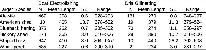
Table 6. Mean length (mm) of catch by species and gear for 2008 in the Roanoke River, NC. ... 57
Table 7. Mean length (mm) of catch by species for (a) boat electrofishing, (b) drift
gillnetting, and (c) set gillnetting for 2009 in the Roanoke River, NC ... 57
Table 8. Bayesian model median estimates of run size by species and year with 90% credible intervals ... 58
Table 9. Bayesian model covariate estimates for 2008 and 2009 with 95% credible
LIST OF FIGURES
Figure 1. Sonar site location in relation to Albemarle Sound and Roanoke Rapids Dam ... 59
Figure 2. A map depicting the location of species composition sampling sites relative to Conine Creek, the split-beam sonar site and DIDSON transect site. Abbreviations refer to the following, (Drift GN) drift gillnetting site, (EF 1–4) boat
electrofishing bank transect sites, (Set GN) set gillnetting site ... 60
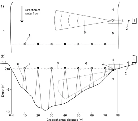
Figure 3. A schematic top (a) and side view (b) of the study site at rkm 64 on the Roanoke River, NC, showing deployment of fixed split-beam and DIDSON transects. Numbers refer to the following, (1) equipment shed, (2) reference stake, (3) split-beam transducer, (4) H-frame, (5) deflection weir, (6) ensonified split-split-beam volume, (7) buoy stops along DIDSON transects, (8) ensonified DIDSON
volume, (9) water level, (10) left bank ... 61
Figure 4. DIDSON images from (a) vertical deployment and (b) horizontal deployment. Panel (a) exemplifies our processing procedure for DIDSON transect data. Shown in (a) are estimates of distance off bottom and fish length of two fish swimming upstream.. ... 62
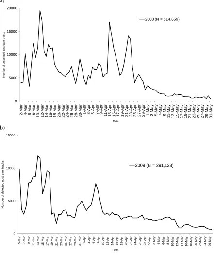
Figure 5. Number of detected upstream tracks from split-beam echosounding in (a) 2008 and (b) 2009. ... 63
Figure 6. Density of total tracked fish targets from (a) 2008 split-beam echosounding, (b) 2009 split-beam echosounding, and (c) 2009 DIDSON transects. Blue shades indicate low densities while red shades indicate high densities. In panel (c), the density plot does not fit the profile exactly, but should be interpreted as extending to the river bottom ... 64
Figure 7. Percent frequency of upstream tracks by hour of day for both 2008 (solid black) and 2009 (dashed gray). ... 65
Figure 8. 2009 Length frequency of fishes from live capture gears (boat electrofishing, and drift gillnetting) compared with estimated length frequency of upstream fishes from DIDSON transect data... 65
Figure 9. Weekly upstream counts from 2009 DIDSON semi-mobile transects. Weekly gage height was obtained from the Williamston USGS gaging station
(#02081054) ... 66
Figure 11. Distribution of fishes across the channel and throughout the water column,
detailed from 2009 DIDSON transect data ... 67
Figure 12. Current velocities at the sonar site with lighter shades indicating low flow areas and darker shades depicting high flow areas ... 67
Figure 13. Water temperature at the sonar site, and discharge from Roanoke Rapids dam in (a) 2008 and (b) 2009. Discharge data were obtained from the Roanoke Rapids USGS gaging station (#02080500) ... 68
Figure 14. Daily estimates of species composition as the proportion of each species captured by all gears in (a) 2008 and (b) 2009. Daily proportions were computed using a 7 d moving average ... 69
Figure 15. Areas sampled (black) and unsampled (gray) by the split-beam sonar in 2008 (top) and 2009 (bottom). Split-beam covered 30% in 2008 and 33% in 2009 of the river cross section, missing near bottom and left bank areas ... 70
Figure 16. 2008 Daily model run size estimates from a Bayesian analysis of split-beam count data using the 2009 mean spatial distribution as a prior for 2008 to account for the lack of DIDSON transect data ... 71
Figure 17. 2009 Daily model run size estimates from a Bayesian analysis of split-beam and DIDSON count data ... 71
Figure 18. Weekly mean log density of θ for select weeks (and days) in 2009. Darker shades indicate higher density, while lighter shades indicate lower density ... 72
Figure 19. Mean log density of θ (left panels) and standard deviation of θ (right panels) for 2008 (top panels) and 2009 (bottom panels). Darker shades indicate higher density for distribution plots and higher standard deviations for variance plots, while lighter shades indicate lower density for distribution plots and lower
INTRODUCTION
Anadromous species are ecologically and economically important fishes. These
species make annual spawning migrations into coastal rivers translocating marine derived
nutrients to freshwater habitats (Helfman 2007). Their presence and abundance in rivers is a
significant indication of biological integrity within the system (Karr 1991). Additionally,
substantial recreational and commercial fisheries exist for these species in both freshwater
and marine systems throughout their range. Historically, alosines(Alosa spp.) supported large-scale fisheries, contributing considerable wealth to the coastal United States
(Hightower et al. 1996; Schmidt et al. 2003; Cooke and Leach 2003). However, the
anthropogenic effects of overfishing, dams, poor water quality and habitat degradation
threaten the abundance of anadromous fish stocks (Leggett and Whitney 1972; Rulifson
1994; Ransom et al. 1998; Limburg and Waldman 2009). Recent efforts aim to restore
populations through stocking (St. Pierre 2003), habitat suitability studies (Burdick and
Hightower 2006; Harris 2010), and improved methods for assessing the current state of
river-specific stocks (Olney et al. 2003; Weaver et al. 2003).
In the western Atlantic Ocean, migratory stocks of anadromous species, namely,
hickory shad Alosa mediocris, American shad Alosa sapidissima, alewife Alosa
pseudoharengus, blueback herring Alosa aestivalis, striped bass Morone saxatilis, and white perch Morone americana use the Roanoke River in North Carolina during spring spawning runs (Menhinick 1991). High flow stretches, freshwater tributaries, and backwater swamps
estuarine and oceanic habitats to feed, grow and mature before homing to their natal rivers as
spawning adults (Jenkins and Burkhead 1993).
Hickory shad are often the first clupeids to enter freshwater drainages for
reproduction, spawning during late winter and early spring in coastal river systems from
Canada to Florida (Mansueti 1962; Richkus and DiNardo 1984; Mitchell 2006). Although
life history of this species is not completely understood, peak spawning is thought to occur
when temperatures are between 12 to 16°C, based on egg collection data from North
Carolina rivers (Sparks 1998; Burdick and Hightower 2006; Harris and Hightower 2007).
River herring (alewife and blueback herring) arrive in early spring and spawn from late
March through June when water temperatures range from 11 to 22°C. (Street et al. 1975;
Walsh et al. 2005). American shad broadcast spawn at temperatures between 14 and 20°C,
during low light and moderate to high flow conditions, and at depths of 1 to 10 m (Walburg
and Nichols 1967; Leggett 1976; Limburg 1996; Hightower and Sparks 2003). Striped bass
are often the last to enter coastal rivers in late spring, and spawn when temperatures reach 17
to 18°C with most outmigrating by June (Trent and Hassler 1968; Olsen and Rulifson 1992;
Carmichael et al. 1998; Kornegay and Thomas 2004).
The predictable seasonal presence of these species in river ecosystems provides an
excellent opportunity to evaluate their status. Traditional monitoring approaches include gill
netting and electrofishing surveys (e.g., Kornegay and Thomas 2004; Thomas et al. 2008).
These annual surveys provide useful relative abundance data, although differences in gear
selectivity and survey catchability may mask actual population changes (Pine et al. 2003).
survey method because of recent advancements in sound technologies (Brandt 1996;
Simmonds and MacLennan 2005). These non-intrusive methods are useful because they can
provide estimates of absolute abundance over short time periods. Furthermore, development
of split-beam sonars have led to the monitoring of fishes in four dimensions (3-dimensions of
space and time; Simmonds and MacLennan 2005).
Riverine hydroacoustic techniques have aided in the assessment and management of
anadromous populations during upstream migrations (spawning runs) to riverine habitats
(Brandt 1996; Simmonds and MacLennan 2005). Fixed-location, side-aspect acoustic
systems are widely recognized for their use in monitoring anadromous salmonids in Alaskan
rivers (Xie et al. 1997; Daum and Osborne 1998; Enzenhofer et al. 1998). These monitoring
techniques enable the enumeration of upstream migrants and provide in-season escapement
estimates used to regulate harvest (Ransom et al. 1998). Specifically, split-beam acoustics
incorporate phase measurements that enable the directional tracking of fish targets in
three-dimensional space, and provide data on the behavior and timing of fish in the beam.
However, the primary disadvantage of this technique is that acoustics data provide little or no
information about fish species or size (Burwen et al. 2003), and often rely on traditional fish
sampling techniques (e.g., gillnetting, electrofishing and trawling) to verify acoustic targets
(Lucas and Baras 2001; Baldwin and McLellan 2008; Boswell et al. 2010).
Further advances in hydroacoustic technology have led to the development of
multi-beam sonars that offer an alternative gear for estimating run size abundance and
characterizing fish behavior during spawning migrations (Maxwell and Grove 2007). A
for naval underwater surveillance (Belcher et al. 2001), has been adopted for fisheries
applications because it provides enough resolution to observe behavioral and morphological
characteristics of fish targets (Baumgartner et al. 2006; Mueller et al. 2010; Burwen et al.
2010). The DIDSON also has advantages over traditional census techniques because of its
ability to image in ambient light conditions and in turbid waters with high levels of
suspended sediments. The system is quickly replacing conventional video cameras and
split-beam sonars to obtain daily counts of migratory fishes (Lilja et al. 2008) because data are
easier to interpret (Boswell et al. 2008; Handegard and Williams 2008), the wider view-field
increases sampled volume providing better spatial coverage (Maxwell and Grove 2007), and
daily counts are both precise and accurate (Holmes et al. 2006). Additionally, estimates of a fish’s length, shape, aspect, direction and swimming speed are obtainable during data
playback (Burwen et al. 2007; Burwen et al. 2010), and most recently estimates of tailbeat
frequencies from DIDSON data may potentially aid species identification (Mueller et al.
2010).
Regardless of the census technique used for assessing upstream migrations or
escapement, objectives include characterizing the temporal and spatial components of the
spawning run (Mulligan and Kieser 1996). Detailed information is generally available about
the temporal component, as field methods often include continuous data collection. The main
limiting factor is the time required for post processing because fish tracking requires
significant time and effort (Enzenhofer and Cronkite 2000; Magowan 2008). Recent studies
have focused on sub-sampling procedures to minimize these difficulties associated with
perspective, census is achieved by restricting fish passage with deflection weirs (Lilja et al.
2008), using multiple horizontal aims to sample the water column (Enzenhofer and Cronkite
2000), or through complete coverage by a transducer array (Daum and Osborne 1998).
However, in river systems where deep channels and fast currents limit the application of
these field techniques, run size models must account for unsampled areas based on assumed
distributions of fish densities in the river cross section (Romakkaniemi et al. 2000; Mitchell
2006; Magowan 2008).
Further investigations into the temporal and spatial expansions are needed to improve
run size model estimates. Establishing an automated approach to fish tracking would
minimize both time and effort and would result in estimates based on all data collected, not a
sub-sampled fraction. Additionally, determining the distribution of fishes using point counts
along a cross channel transect would aid the spatial expansion of fish counts to unsampled
areas. Both efforts would improve the timeliness and accuracy of population assessments to
evaluate management and restoration objectives.
This paper is part of an ongoing effort to improve the methodology of estimating run
sizes using hydroacoustic survey methods on the Roanoke River, NC. The objectives were to
(1) obtain daily counts of upstream migrants using a fixed location split-beam sonar, (2)
detail the distribution of fishes in the river cross section using DIDSON point counts along a
transect, (3) spatially integrate the two data types using a Bayesian hierarchical model which
expands split-beam counts based on the cross channel distribution, and (4) use information
from concurrent gill netting and electrofishing to produce species-specific run size estimates
restoration efforts as part of a Federal Energy Regulatory Commission (FERC) relicensing
process for hydroelectric dams operated by Dominion Power. The methods should prove
useful in similar riverine systems where species-specific run sizes are desired.
METHODS Study Area
The Roanoke River flows southeast from Virginia through North Carolina to its
confluence with western Albemarle Sound, NC. Roanoke Rapids dam (rkm 221), a
hydroelectric power source, limits the upstream migration of anadromous fishes (Rulifson
and Manooch 1990). Hydroacoustics monitoring occurred at rkm 64 (Figure 1); this site is
ideal for detailing spawning run abundance and timing given its location near the entrance of
the Roanoke River. Furthermore, the site is located upstream of alternate upstream routes
(such as Conine Creek, Figure 2), thus migrants were forced to swim past the study site in
order to reach their preferred spawning habitat (Figure 2).
This location was also selected because the riverbed profile was ideal for fixed sonar
deployment (see Enzenhofer and Cronkite 2000). River width at the site was ~80 m. From
the right bank the bottom slopes gradually to a thalweg depth of 12.5 m, followed by a steep
upslope on the left bank (Figure 3). The site had laminar flow and was well downstream of
known spawning areas; therefore, fishes actively migrated past this location without milling.
Hydroacoustic Monitoring
Run size estimates of anadromous fishes were based on data collected with two major
gears: a split-beam sonar and a DIDSON (multi-beam) sonar (Figure 3). Acoustics data were
species composition estimates on a weekly basis, drift gill nets and boat electrofishing
occurred during each year.
Split-beam.—Split-beam acoustic systems enable directional tracking of fish targets in three-dimensional space. Transducers are split into four quadrants and transmission
occurs simultaneously in all quadrants, but return signals are retrieved at independent
intervals. This enables the system to estimate three dimensional position by computing shifts
in the phases from one quadrant to the next of a returned ping (Enzenhofer et al. 1998).
Monitoring was done continuously using a calibrated 430 kHz Biosonics 7° circular
split-beam echosounder (Biosonics, Inc.). The unit was mounted on a fixed H-frame that
enabled in-situ adjustments of pan and tilt axes. To limit fish from swimming in the near field of the beam, a weir was installed 0.5 m downstream of the mount, and extended 1.5 m
beyond the face of the transducer (Figure 3). The weir was a 2.5-m high panel of 5-cm
square construction mesh designed to guide upstream migrants into the ensonified region. We manually adjusted the weir’s position along the bank in response to changing river flows
and transducer placement. Sound transmission settings were: 0.2 ms pulse width, 10 pings·s-1
pulse repetition rate and -70 dB sensitivity threshold, a level that recorded enough
backscatter to scrutinize echograms for fish targets. We reduced transmission power to -14
dB, decreasing the signal intensity to below the hearing range of Alosa ssp. and thus, minimizing their avoidance of our gear (Gregory and Clabburn 2003). A laptop, operating
DTX visual acquisition software (Biosonics Inc.), logged data in 20-minute files and stored
them on an external hard drive. Data collection occurred 24 h·day-1 except during field trials,
quality, we aimed the transducer daily to capture a ~45 m range, which was perpendicular to
the current with a near bottom orientation. Daily metrics recorded at the site included sonar
heading, pitch and roll, river width, depth of the transducer, distance of the transducer to the
waterline and to a reference stake, maximum river depth, and water temperature. We moved
the transducer up or down the bank during changes in river stage to keep it submerged.
DIDSON.—The standard DIDSON is a multi-beam imaging sonar that uses an array of lenses to create a 14° vertical by 29° horizontal beam (Belcher et al. 2001). The system
operates at two frequencies (1.1 and 1.8 MHz), each with an associated range and resolution.
In high-frequency mode (1.8 MHz), which is restricted to shorter ranges (<15 m), 96 beams
create a 0.3° horizontal resolution. In low-frequency mode (1.1 MHz), the beams are
reduced to 48, which sacrifices resolution but increases sampling range to approximately 30
m. An image is built sequentially by eight sets of 12 beams that transmit simultaneously to
reduce cross-talk between beams. DIDSON images can be analyzed to obtain estimates of
fish length, direction (i.e., upstream or downstream) and behavioral characteristics (Burwen
et al. 2007), however the data are arrayed in 2-dimensions (X and Y with no resolution in the
Z dimension), and consequently 3-dimensional position information is not available (Belcher
et al. 2001).
To detail the distribution of fishes across the river channel, we collected data using a
DIDSON at several fixed points along a cross channel transect, from 5 March to 27 May
2009. Transects occurred 30 m downstream of split-beam echosounding, a location that had
similar bottom topography. We placed a buoyed anchor every 10 m across the river to
data collection. A spreader lens, that increases the vertical dimension of the beam from 14 to
28°, was used to increase the volume sampled. At each anchor location from the left to right
bank, the DIDSON was mounted vertically on a pole, secured on the stern of the vessel, and
lowered to an operational depth beneath the water surface with the X axis of the beam
parallel to the flow. We used a stern anchor to further steady the vessel, and recorded a
5-minute file with the smallest window start and a suitable window length that captured the
bottom at a fixed depth. The depth did not exceed 10 m at any of the deployed locations,
enabling high resolution data collection. Transects occurred 3 d a week and the start time
was randomly selected and restricted to daylight hours (08:00 to 19:00).
Current Profiling.—We measured water velocities one time at the sonar site on 26 May 2009 using a 2 MHz acoustic Doppler current profiler (Aquadopp; Nortek AS). The
Aquadopp profiler contains three adjacent acoustic beams angled at 25° enabling users to
obtain current velocities in user defined cells (http://www.nortek-as.com). We deployed the
profiler just beneath the water surface on a pole mounted to the bow of a stationary vessel.
We operated this equipments along the same cross channel transect as DIDSON data, but
obtained measurements on 5 m intervals across the river. Using a 0.2-m blanking distance,
and 0.1-m cell interval, we recorded a 2 min file averaging measured velocities on a 30 s
time interval (i.e., 4 data points per 5-m deployment). Aquadopp data were averaged by
cross channel grid cell to be included as a covariate in Bayesian modeling (see Bayesian Run
Acoustic Data Processing
To obtain fish counts of upstream migrants, acoustics data were imported and
processed in Echoview (version 4.5, SonarData Pty., Ltd.). Raw split-beam data were
converted to single target echograms (STE), which display individual echoes based on
angular position and target strength criteria, and are useful to select fish targets by
eliminating noisy backscatter. Within STEs, fish tracks were identified automatically using a
dynamic tracking algorithm that selects a series of echoes with a consistent trajectory in both
position and velocity (Blackman 1986). Specific alpha and beta parameters, which allow
position and velocity to vary within a track path, were adjusted to maximize tracking
accuracy (see Magowan 2008). Fish tracking was automated using the scripting module in
Echoview because of the large volume of data (>85 d·season-1) to be processed. The script
cycled on 24 h datasets, processing 8 h of data at a time, and exported a tracked echoview file
and metrics of each fish tracked (script available, contact author). These metrics were used
to analyze each track and included date and time, target strength (compensated for position within the beam), horizontal direction, tortuosity (a fish’s actual trajectory compared to a
linear path), duration in beam, and angle of deviation from beam axes. Tracks were
separated into upstream and downstream constituents based on radial measurements of
direction. Those with a horizontal trajectory between 225 and 315° were classified as
upstream based on our transducer orientation.
Further processing was restricted to upstream migrants because downstream tracks
include false targets (e.g., woody debris). Track position was calculated to determine a fish’s
for spatial expansion, tracks were overlaid onto the bottom profile, created from the
maximum gauge height observed in both years. An estimate of range from shore was
calculated from a reference stake (spatial benchmark; Figure 2) used in both years because
transducer position changed with river stage. Tracks from an entire field season were plotted
and manually scrutinized to eliminate erroneous data, created by false tracking of surface or
bottom reverberation.
To account for the inclusion of false targets in upstream tracks, we determined a
misclassification rate from a small subset of the automatically tracked files. We randomly
selected and examined twelve 20-min data files, four from each month in 2008. Files were manually scrutinized to reclassify automatically detected tracks into ―fish‖ and ―noise‖
classes and calculate a misclassification rate as noise tracks/total tracks. We used the
misclassification rate to adjust modeled run size estimates.
To determine the distribution of fishes across the river channel, raw DIDSON transect
data were manually processed with the DIDSON display and control software version 5.23
(Soundmetrics, Inc.). Unlike a side-aspect deployment, contrast between a fish and
surrounding background was high because a vertical deployment does not contain substrate
throughout its range (Figure 4). Therefore, fish did not blend with the substrate, and
DIDSON images were played back at 20 frames·s-1 (2X real time), until an upstream fish
target was observed. Stepping through frame by frame, a single frame was selected to obtain an estimate of a fish’s length and distance off bottom using the manual fish measuring
unformatted text files and a JMP (SAS Institute Inc., version 8) script was developed to
import needed variables into a workable format (Steve Williams, personal communication).
Fish processed during DIDSON playback were spatially integrated into the bottom
profile with split-beam data as discussed earlier. To position DIDSON fish in the river
cross-section, the distance off bottom (elevation, Y) was used in combination with transect buoy
location (a discrete measure of range from the left bank, X). Although the DIDSON transect
was downstream of the split-beam sonar site, the bottom topography at the two sites were
similar and we assumed the cross sectional fish distribution was consistent at both locations
(Figure 3).
Species Composition
Species composition sampling was used to (1) document the timing of species
migrations, (2) examine the size distribution of target fishes, and (3) partition modeled fish
counts into species-specific run size estimates. Sampling protocol consisted of boat
electrofishing and drift gillnetting 5 d a week (Monday-Friday). We combined these live
capture techniques to identify fish assemblages along the banks (electrofishing) and in the
channel (gillnetting), based on the advantages of each gear in selected habitats (Casselman et
al. 1990). Daily sampling was separated into AM and PM sampling times and the gear order
was alternated systematically (i.e., gillnetting in the AM and electrofishing in the PM one
day, electrofishing in the AM and gillnetting in the PM the next; Magowan 2008).
Drift gillnetting occurred 4.3 rkm upstream of the sonar site to minimize disturbance
of upstream migrants (Figure 2). Effort included two drifts of three different mesh sizes (7,
Jenkins and Burkhead 1993). All drifts occurred perpendicular to the flow over the same 200
m river stretch, and the order nets were set was rotated systematically (e.g., 7, 10, 14 cm one
day, 10, 14, 7 cm the next; Magowan 2008). Gill nets were designed to sample the entire
water column, and were 23 m long by 3.7, 4.9, or 7.3-m deep depending on river stage. Fish
captured were identified, examined to determine sex, measured (max TL) and released. Fish
orientation (upstream or downstream), capture location (top or bottom of net), and
reproductive condition (e.g., running ripe, spent) was indicated when possible. Reproductive
condition was determined by applying light pressure along the abdomen towards the vent
(Acolas et al. 2006). Fish producing eggs or milt were considered running upstream, and fish
that were visually emaciated were thought to be outmigrating and spent. Catch per unit effort
(CPUE) was calculated by set (the catch from all three mesh sizes) as #fish·set-1 because gill
nets are a size selective gear (Hubert 1996).
Boat electrofishing was conducted using a Model 7.5 Generator Powered Pulsator
(GPP) Smith-Root electrofishing system. Alongshore transects occurred at two locations, 0.7
and 1.8 rkm upstream of the hydroacoustic site (Figure 2). We characterized electrofishing
sites (E1 and E3) as cut banks and (E2 and E4) as flat banks to determine if anadromous
fishes had a bank preference during migrations. The cut banks formed on the outside of
channel crossovers, while flat banks were on the inside of shallow bends (Figure 2). A
sample in 2008 was comprised of four 900 s transects, moving in a downstream direction
along each bank at both locations with one netter. In 2009, effort was reduced to two
transects, one bank chosen randomly at each location because of large catches in 2008. The
amperes, a non-lethal output power. Banks were fished in random order. Fish captured were
initially held in an aerated tank until completion of a transect, and were then identified,
examined to determine sex, measured (max TL), checked for reproductive condition and
released. CPUE was calculated by averaging daily catch at all electrofishing transects as
(#fish·900s-1).
We included set gill nets as a species composition sampling gear in 2009 because of
its potential to (1) provide directional information of fishes migrating along the riverbanks,
and (2) identify species actively migrating along the banks. Sets occurred between
electrofishing and drift gillnetting sites, on the downstream side of a point bar; a location that
provided refuge from the high flows associated with the deeper mid-channel (Figure 2). Nets
were the same used for drift gillnetting, and dimensions selected based on river stage.
Anchors grounded the net perpendicular to the current with buoy floats marking their
location. We used a 15-min soak time and set nets during daylight hours (i.e., 8:00 to 19:00).
Fishes captured were identified, examined to determine sex, measured and released – noting
orientation (upstream or downstream) and reproductive condition when possible.
Catch data from all gears were restricted to fish swimming upstream, determined
primarily from reproduction condition and secondarily from directional information obtained
only in gill net sampling. We computed a series of statistical tests (e.g., t-test, ANOVA) to
test each species for gear-specific differences in size; and total catch from steep versus
shallow sloping banks (Zar 1996). All tests were controlled for type I error at an α = 0.05
To account for the magnitude of nonmigratory fishes (i.e., resident species), we
estimated the average number of upstream migrants per day at times when anadromous fishes
were absent from sampling (i.e., after outmigration; Banneheka et al. 1995). We removed
this average resident contribution from daily estimates obtained with our run size model. To
account for freshwater fishes making a potamodromous migration (i.e., gizzard shad
Dorosoma cepedianum, white catfish Ameriurus catus, striped mullet Mugil cephalus) we included them in daily species composition for migratory fishes. We smoothed estimates of
daily composition of migratory fishes using a seven day moving average, summing on the
sample day d, and averaging with sample days, d-3, d-2, d-1, d+1, d+2, d+3 (Acolas et al. 2006; Mitchell 2006; Magowan 2008).
Bayesian Run Size Modeling
We used a Bayesian modeling framework to estimate annual run size from the
combination of split-beam and DIDSON count datasets. We chose this analysis pathway
because of the Poisson nature of our point counts, the spatial correlation in our two data
types, and our uneven sampling design, all of which are difficult to analyze with frequentist
statistics under parametric assumptions (McCarthy 2007; Link and Barker 2010). Therefore,
we implemented a hierarchical Poisson regression model, which accounted for the space and
time structure of our count data, to estimate daily run size by season.
Bayesian statistics are gaining popularity because of their flexibility to deal with a
spectrum of study designs of varying complexity, and diverse application. The framework
includes assigning prior knowledge about the distribution of model parameters, which are
Markov Chain Monte Carlo method (MCMC) is a simulation approach to estimate the
posterior distribution (see Gilks et al. 1996), and has performed well over alternative
simulation approaches (Newman et al. 2009). McCarthy (2007) defines a Markov chain as a
set of random numbers drawn from the posterior distribution in which the value of each is
conditional on the previous. Replicating the chain, an easier feat with modern computing,
assures convergence on a stable posterior distribution (Cowles and Carlin 1996). The results
yield estimates of mean, variance and percentiles of the distribution (Link and Sauer 2002).
Hierarchical models provide a platform for incorporating complexity that is not easily
analyzed with other statistical approaches (Rivot et al. 2004; Sauer et al. 2008). Using a
hierarchal model gave us the flexibility to jointly analyze our two data sources (split-beam
and DIDSON) and to incorporate spatial and temporal correlation as well as covariates. This
framework enables us to model run size based on observed trends in the dataset (Link and
Sauer 2002).
We delineated a spatial grid in the river cross section, with individual cell dimensions
1-m deep by 2-m wide. We modeled the expected count in cell s on day k using the log
linear model,
log[λk(s)] = μk+ x(s)'β+ θ(s) + αk(s)
where μk is the random effect for day k, x(s) are the spatial covariates determined by the
position of a cell in the cross section, β are the corresponding regression coefficients, θ(s) is a
random effect to capture spatial trends not explained by the covariates, and αk(s) captures
daily variation in the spatial distribution. We analyzed the split-beam and DIDSON data
yk(s) ~ Poisson(θE(s)λk(s))
where yk(s) is the number of fish recorded in split-beam cell s on day k, E(s) is the amount of
time (proportion of day) that cell s was under observation with E(s) = 0 for cells outside the beam dimensions, and θ is a bias term to account for systematic difference between the two
types of counts. We excluded cells sampled less than 50% of the time by the split-beam in
each season to minimize the bias from undercounting in those cells. To clarify, retained cells
contained at least one tracked fish on more than 50% of the days in a single season.
Therefore, within each season, we assumed the intensity was constant in split beam grid cells
that were retained.
Simultaneously we modeled,
zk(j) ~ Poisson(F(j)∑ni=1 W(j,s)λk(s))
where zk(j) is the number of fish recorded in DIDSON cell j, F(j) is the amount of time this
cell was under observation, and W(j,s)is the area of overlap between DIDSON cell j and split-beam cell s.
We expected spatial correlation in cell counts across the river channel because of the
regional clustering of our data. Therefore, we modeled extra Poisson variability to smooth
neighboring cells that shared a border with the cell of interest (Best et al. 1999). We do this
using a conditionally autoregressive (CAR) model for the θ(s)(Banerjee et al. 2004). The CAR model can be defined through its conditional distribution for θ(s)given all other values
as,
θ(s) | θ(t), t≠s ~ Normal(ρU(s), ζ2/m(s))
spatial neighbors, and ζ2
controls the variance. This leads to a multivariate normal
distribution for the vector θ = [θ(1),...,θ(n)]'~N(0, ζ2[M-ρD]-1), where M is diagonal with diagonal elements m(s) and the (s,t) element of D is one if s and t are adjacent and zero otherwise. The daily random effects αk(s) are assumed to be constant within week, with
independent CAR priors for the weekly spatial processes with association parameter ρα and
variance ζ2
α. We modeled the daily random effects μk using the autoregressive time series
model μk ~N(δ μk-1,η2) , where δ ε[-1,1] controls the strength of autocorrelation and η2
controls the variance.
To implement our fully-Bayesian model, we specify the following priors. We assume the regression coefficients β have uninformative normal priors N(0,102). The bias term θ has
a Gamma(0.01,0.01) prior, parameterized to have mean one and variance 100. The CAR covariance parameter have priors ρ, ρα ~ Uniform(0,1) and ζ2, ζ2α~ InvGamma(0.5,0.005), as
recommended by Kelsall and Wakefield (1999), and δ ~ Uniform(-1,1) and η2
~
InvGamma(0.5,0.005).
Down-looking DIDSON data were only collected in 2009 so daily split-beam counts
in 2008 were modeled simultaneously with the 2009 data using the similar model, log[λ*k(s)] = μ*k+ x(s)'β*+ θ* (s) + α*k(s),
where λ*k(s) was the expected count for cell s on day k of 2008, and μ*, β*, θ*, and α* had
the same interpretations as μ, β, θ, and αin the 2009 model. The priors for μ*, β*, θ*, and α*
were the same as the 2009 priors, except that to pool information across the two years, the
After review of the literature, we selected covariates to include in the model that were
either measured during this study or easily obtainable from available riverine data stations.
The model was divided into a space and time context, which is similar to the variables
associated with anadromous fishes on spawning runs (e.g., timing, flow). Spatially, we chose
distance off bottom and distance from bank as additive covariates on observed counts.
Fishes making active migrations in riverine systems tend to be bank and bottom oriented –
areas that are usually associated with low flow velocities (Witherell and Kynard 1990; Daum
and Osborne 1998; Enzenhofer and Cronkite 2000). Temporally, river discharge and water
temperature were covariates chosen to predict abundance and timing of upstream migrants
(Mitchell 2006; Magowan 2008).
The model was fit using WinBUGS 1.4.3 (Spiegelhalter et al. 2003), a freely
available statistical package that is commonly used for Bayesian analysis. This user-friendly
program applies MCMC methods to obtain samples from the posterior distributions of model
parameters. It provides estimates of precision for parameter estimates such as credible
intervals (the Bayesian analog of confidence intervals). We executed the Markov chain using an initial ―burn in‖ (transitory period that is excluded so that initial values do not affect the
final results), then replicated the chain to assure convergence (Brooks and Gelman 1998).
The purpose of replication is to give WinBUGS multiple starting points (initial values) along
each chain, and we tested for convergence on the posterior distributions using Gelman-Rubin
(G–R) diagnostic embedded in WinBUGS (Spiegelhalter et al. 2003). The G–R is a
diagnostic statistic that compares the variation within chains to variation across chains.
To finalize our objective, we computed species specific run size estimates as,
i i
i CS
Nˆ ˆ ˆ
where on day i, Nˆi is the estimated number of fish of a particular species, Cˆiis the
hierarchical model estimated count of upstream fishes, and Sˆiis the proportion of the
estimated count comprised by that species in the river cross section, estimated by the 7 d
moving average of live capture gears described earlier.
RESULTS
Hydroacoustic Monitoring
In 2008, 514,659 upstream tracks were detected passing the split-beam site from 2
March to 31 May. Peaks in daily upstream passage occurred in mid March, and mid to late
April with upstream passage decreasing substantially by mid May (Figure 5). Mean
split-beam track distance from shore was 16.05 m with 75% of tracks within 24.42 m (Figure 6).
In 2009, 291,128 upstream tracks were detected from 5 March to 27 May (Figure 5). Peaks
in daily upstream passage were less pronounced, but were still evident in early to mid March,
and mid April (Figure 5). Mean track distance from shore was 14.94 m with 75% of tracks
within 22.32 m. In both years, upstream passage was highest during morning (06:00 to
10:00) and evening (17:00 to 20:00) hours (Figure 7).
A total of 929 DIDSON fish images were measured from 36 DIDSON transects
during the 13-week 2009 season. Fish were easy to identify during playback and direction of
travel (upstream/downstream) confirmed from their rheotactic swimming behavior. We
interfere with fish measuring and this view still provided morphological information (Figure
4). The starting range for each DIDSON file (window start setting) was the closest available
for the chosen window length. Window length was either 2.5 or 5 m at shallower sites
depending on river stage, and did not exceed 10 m at deeper sites. Aspect angle of measured
fish (with 0° being in the center of the beam) ranged from -31.30 to 46.30°, with an average
of 0.66°, an expected result because migrating fish made distinct upstream movements and
remained perpendicular to the beam while ensonified. Estimated fish lengths ranged from
5.90 to 90.80 cm, with a mean length of 32.98 cm and 90% measuring less than 45.10 cm.
Estimated lengths differed as a function of cross channel location, with smaller fishes along
the flat bank (i.e., 70-m; Figure 3) compared to mid channel or cut bank sites (n = 929, F =
12.57, P < 0.0001; Table 1). Generally, length frequency from all DIDSON transects
matched well with length frequencies of total catch from our species composition gears in
2009 (Figure 8).
Similar to 2009 split-beam counts, DIDSON transects identified a peak in fish
passage during mid-March and early April, with lowest passage in mid to late May (Figure
9). Weekly upstream split-beam counts were significantly correlated with weekly DIDSON
counts (n = 13, r = 0.8159, p = 0.0007; Figure 10). Fish were generally bottom and shore
oriented, with 75% within 1 m of the bottom and 82% within 20 m of each bank (Figure 6c).
More specifically, fish passage over the season differed across the channel (n = 82, F = 6.31,
p < 0.0001; Figure 11), with a Tukey’s test to compare means suggesting that passage tended
to be higher within 20 m of each bank than in the mid channel. Additionally, more fish
statistically significant. Diel migration patterns were not discernible because DIDSON data
collection only occurred during daytime.
Current velocities on 26 May 2009, ranged from zero to 0.60 m·s-1 with swifter flows
(> 0.40 m·s-1) in the mid-channel and lowest flows (< 0.20 m·s-1) detected near bottom and
along shore (Figure 12). The flat bank had below average flows (0.40 m·s-1) that extended 30
m into the channel, while the cut bank has high flows within 20 m.
Water temperatures over the field seasons were typical for the Roanoke River in
spring, with cool temperatures in early March (< 9°C), followed by a steady increase to
warmer temperatures in April (~15°C) and in late May (22°C; Figure 13). Periodically, daily
temperatures held steady or decreased slightly when large rain events occurred or discharge
released from the dam exceeded 295 m3·s-1. Discharge in 2008 averaged 196.66 m3·s-1,
starting low in March (< 109 m3·s-1), and increasing in mid April, a preplanned annual release
schedule to promote the active migration of anadromous fishes (Figure 13). In early March
2009, water temperatures were 6°C, and stayed cooler because of a large rain event on 1
March, which forced peak discharge (> 566 m3·s-1). An increase in rainfall in early March
2009 enabled the early release of preplanned migratory flows in late March (Figure 13).
There was roughly a 1.5-d lag between released water from Roanoke Rapids Dam (rkm 221)
and an increased river stage at the study site (rkm 64).
Species Composition
We captured 27 species using drift gill netting, set gill netting, and boat electrofishing
(Tables 2 and 3). Fish assemblages differed by habitat type, with resident species comprising
mid-channel, representing 94 and 95% of gill net catches in the two years respectively.
Generally, electrofishing CPUE was relatively higher than gill net CPUE, except for
American shad, which were captured more efficiently with drift gill nets in both years
(Tables 4 and 5). Striped bass, white perch, and river herring were the most abundant target
species ranging from 7 to 19% of the total catch, while hickory shad and American shad
accounted for less than 4% of total catch in both years.
In both years, the spawning migration began with hickory shad and alewife in early
March, with blueback herring arriving in late March to early April, and American shad,
striped bass and white perch following in mid to late April and in early May (Figure 14). In
2009, the arrival of anadromous fishes was early, with most fishes present in the first week of
March, except blueback herring, which arrived during week three. The early arrival
coincided with a high discharge release of 546.52 m3·s-1 on 3 March from Roanoke Rapids
dam (Figure 13), causing a significant rise in river stage (~1.13 m increase) at the study site
on 5 March. Despite the early arrival, max CPUE for blueback herring, striped bass, white
perch and American shad did not peak until April, when temperatures were 14 to 20°C
(Table 5).
In 2008, both drift gillnetting and boat electrofishing daily CPUE (for the entire
catch) was significantly correlated with detected upstream tracks (n = 65, r = 0.7568, p <
0.0001, and n = 62, r = 0.5132, p < 0.0001, respectively). More specifically, boat
electrofishing CPUE for resident fishes was not significantly correlated with detected
upstream tracks (n = 62, r = 0.1559, p = 0.2264), suggesting that pulses of detected tracks
was significantly correlated with detected upstream tracks (n = 59, r = 0.6870, p < 0.0001),
but boat electrofishing CPUE was not (n = 60, r = 0.0154, p = 0.9069).
Drift gill nets captured 11 species, with highest catches composed of alewife in both
years. Maximum CPUE for drift gillnetting, caused by strong pulses of hickory shad and
alewife, occurred on 12 March in both years when water temperatures were 12 to 13°C.
Mean CPUE was similar for the 2008 and 2009 field seasons at 2.6 and 2.2 fish per 200 m
drift respectively. The 7-cm mesh size was the most productive, capturing mainly river
herring and occasionally smaller hickory shad and striped bass and accounting for greater
than 80% of all drift net catches in the study. The 10-cm mesh size targeted hickory shad,
American shad, and striped bass, while the 14-cm mesh size was the least productive,
capturing less than 4% of the total drift net catch, mainly few large striped bass and fewer
American shad.
Boat electrofishing captured 26 species, detailing a more diverse fish assemblage
along the riverbanks with a mixture of anadromous and resident species. Maximum CPUE
for boat electrofishing, dominated by abundant catches of striped bass and white perch,
occurred around 21 April when water temperatures were 16°C. Average CPUE was slightly
lower in 2008 (23.2 fish·900s-1) than in 2009 (30.3 fish·900s-1). Generally, alosines
responded poorly to electrical shock, often resulting in erratic movements, and marginal
buoyancy, thus making them difficult to capture. Conversely, the large swim bladder of
In 2008, catch of anadromous fishes using electrofishing was highest along the cut
banks, but mean log CPUE was not significantly different between the two bank types over
the season (n = 57, t = -1.18, p = 0.24). In 2009, catches were significantly higher along flat
banks than cut banks (n = 60, t = 4.31, p < 0.0001).
Set gill nets captured 16 species, identifying fishes actively migrating along a flat
bank. Catches from set gill nets were comparable to the other sampling gears, documenting
similar timing and abundance of anadromous targets (Table 5). Most notably, set nets
appeared advantageous over drift nets because they captured higher abundances of striped
bass and white perch while maintaining the capture of river herring and hickory shad.
Anadromous targets represented a majority of set net catches, while resident species
accounted for 28% of the total catch. Additionally, this gear identified a potamodromous
migration of white catfish, a non-target species in May.
The length range of captured anadromous fishes was typical of these species in
southeastern rivers. Generally, mean length of fishes captured in gill nets were higher than
electrofishing captures, resulting from the size-selectivity of our gill nets (Tables 6 and 7).
This gear effect was most evident for river herring, as the mean length captured with gill nets
was significantly higher than the observed mean length from boat electrofishing in 2008 (n =
1093, t = 17.57, p < 0.0001) and 2009 (n = 328, t = 14.91, p < 0.0001). Although this size
selectivity was observed for most other anadromous fishes, except for American shad, small
Bayesian Run Size Modeling
Sampled area by the split-beam was relatively consistent in both years, covering 30%
of the cross-sectional area in 2008, and 33% in 2009 (Figure 15). We eliminated cells
sampled less than 50% of the time by the split-beam over the entire season to minimize the
bias from undercounting in those cells. Furthermore, excluded cells were often on the fringes
of the beam, and at its farthest ranges, an area usually associated with decreased detection
probabilities. It was evident from placing raw count data in the river cross section grid that
split-beam coverage was lacking near the substrate across the entire sampled range (Figure
15). However, the addition of DIDSON data from cross channel transects increased our
coverage of the left bank (an area unsampled by split-beam echosounding), and near bottom
areas across the entire channel (Figure 3).
We ran two independent MCMC chains, each with 100,000 iterations, discarding the
first 25,000 samples in each chain as burn-in. To assure convergence on posterior
distributions we monitored the G–R statistic provided in WinBUGS, finding it was nearly 1.0
for all parameters, indicating that the model converged on stable posterior distributions.
Modeled run size estimates were relatively similar in both years, despite differences in raw
split-beam counts. We present median estimates (instead of mean) with 5% and 95%
credible intervals because daily means were skewed towards the upper quantiles. We
decreased expected counts by 7.28%, based on a measured misclassification rate of detected
tracks assumed to be equal in both years. In 2008, our hierarchical Bayesian model
estimated total run size as 1,485,958 upstream migrants (90% credible interval 900,601 to
tracks with a 90% credible interval of 997,375 to 2,083,262 (Figure 17). Species specific run
size estimates and credible intervals are shown for both years in Table 8.
We modeled the two years simultaneously to account for the absence of
down-looking DIDSON data in 2008. Given the enhanced spatial coverage from the combination
of the two sonars in 2009, we were able to account for variation in spatial density by week
(Figure 18), leading to narrower credible intervals. In 2008, DIDSON transect data were
unavailable; therefore, to account for this we pooled the spatial density across both years,
conditioning 2008 priors on the 2009 mean spatial distribution. As a result, the 2008 density
surface represents the spatial deviance from 2009. Given the spatial pattern of split-beam
tracks was similar for both years (higher densities near shore, Figures 6a and 6b) the variance
in spatial correlation was less in 2008 because 2009 absorbed a significant amount of the
variability. Lastly, standard deviations were notably larger in cells unsampled by either gear
(Figure 19).
Spatial and temporal effects were strongly associated with expected daily counts in
both years. The spatial association parameter from the CAR model was nearly 1.0 in both
years (Table 9), indicating strong clustering of cells with high and low expected counts. This
was further explained by the significance of spatial covariates on mean log densities (Table
9). In 2008, distance from bank and distance off bottom were significant parameters,
whereas in 2009, distance from bank was significant and distance off bottom was marginally
significant (Table 9). Therefore, our modeling suggests that cells located closest to the bank
also found a strong temporal correlation in both years, suggesting expected counts across
days were similar. Lastly, flow and water depth were not significant covariates in our model.
Although averaged current velocity (flow) within each cell was not a significant
covariate, we explored the relationship of current velocities on spatial density outside the
context of our model. Using measured mean cell velocities and associated mean spatial
density estimates from our model, we found these variables to be significantly correlated in
both 2008 (n = 446, r = -0.3177, p < 0.0001) and 2009 (n = 446, r = -0.6611, p < 0.0001).
DISCUSSION
Hydroacoustic Monitoring
Hydroacoustics provides a complete noninvasive census method for obtaining counts
of upstream migrants over a sampled volume of water in river systems (Enzenhofer and
Cronkite 2000). Ideally, one or more transducers are set up on each shoreline to minimize
unsampled zones in the river cross section (Daum and Osborne 1998). However, a spatial
expansion of counts is necessary when a portion of the river channel is acoustically
unsampled (Romakkaniemi et al. 2000). The expansion model extrapolates fish counts based
on the distribution of upstream migrants occupying the unsampled area. In this study, a fixed
side-aspect split-beam sonar covered 30-33% of the river cross-section, but DIDSON
transects provided information about the overall pattern in fish density across the channel.
Our Bayesian hierarchical model was effective in combining the two information sources,
not only to estimate annual run size, but also to describe spatial and temporal patterns in
Deploying a DIDSON on a cross channel transect enabled us to determine that
upstream migrants were shore and bottom oriented during the spawning run. Our result was
consistent with previous studies of spawning runs on the Roanoke River, which found similar
spatial patterns using side aspect split-beam echosounding (Mitchell 2006; Magowan 2008).
More specifically, we observed a significantly higher count within 20 m of each bank, even
without accounting for the smaller proportion of sampled volume at these locations (a
function of beam geometry and sampled depth). This was an expected result, as these areas
had slower current velocities because of river topography and hydrology (Chanson 1999).
This is also physiologically intuitive, as fishes often migrate in low flow areas whenever
possible (Standen et al. 2004), presumably to budget for the energetic demands associated
with ascending rivers to spawn (Leonard et al. 1999). Furthermore, this migratory pattern is
consistent with the behavior of spawning salmonids, which have similar anadromous life
histories. In the Chandalar River, Alaska, 90% of chum salmon traveled within 26 m of each
bank (mean river width was 128 m), and 98% were detected in the lower half of the beam
(Daum and Osborne 1998). In the Fraser River, Canada, a mobile survey of sockeye salmon
determined that upstream migrants were bottom and shore oriented (Chen et al. 2004).
Hydroacoustic transect surveys have several advantages over direct capture
techniques. This gear is not size selective, at least over the size range of interest. There are
no issues regarding bycatch or incidental mortality that might arise with net sampling.
Hydroacoustic samples also require less time and effort to obtain, although the time required
for processing must be considered. The transect approach used here (a series of fixed points
vessels under power (Mitson and Knudsen 2003), especially when transecting rivers in
shallow water environments because of associated mechanical engine noise (Xie et al. 2002).
Xie et al. (2008) found salmonids (Oncorhynchusspp.) initiated a lateral avoidance behavior when within 4 m of a vessel propeller, but were unaffected at a distance of 7 m. To limit this
affect, we used an anchored deployment without engine power, and movement of the vessel
while collecting data was negligible, presumably minimizing fish avoidance of our sampled
volume. Transects during this study occurred during daylight hours and we cannot assess the
possibility that fish distribution may have changed at night. Although this is plausible,
previous studies on the Roanoke River found a consistent spatial pattern in diel catch data for
anadromous fishes (Mitchell 2006), and we found fish passage rates (as measured with
split-beam echosounding) to be less during nighttime, a finding also consistent with preceding
studies (Mitchell 2006; Magowan 2008). Additionally, we randomly chose transect start
time to minimize time biases associated with fish passage estimates during daytime.
Additional limitations of mobile surveys include the personnel and time required to
operate the gear and collect the data. The duration of transects in our study was limited by
the demand to accomplish other field tasks. Lilja et al. (2008) recommended sampling a
minimum of 10-min·h-1 to estimate total upstream passage during the spawning season.
However, the objective of our cross channel transect was not to estimate abundance, but to
detail the spatial trends of fish targets during their upstream migrations to improve run size
model estimates. Although we acknowledge that increasing the sampling time and frequency
in 2009 was relatively consistent on a weekly basis, and our modeling accounted for small
distributional changes by week.
An analysis of fish size distributions in the river-cross section found that fishes
located near the flat bank and along the bottom tended to be smaller. There are several
biological principles that may explain these observed trends. First, a predator-prey
interaction may exist in which larger piscivorous fishes (e.g., striped bass) are forcing smaller
fishes (i.e., river herring and white perch) to seek refuge from predation in shallower habitats.
Although we were unable to test this hypothesis, species composition sampling showed that
river herring were found in higher abundance along the banks than in the mid channel.
Walter and Austin (2003) found that alosines and white perch peaked in striped bass diets
during spring spawning months in Chesapeake Bay, MD. Alternatively, specific habitat
selection of smaller fishes may be a direct response to avoid areas with high current
velocities. A reasonable hypothesis considering these species (e.g., clupeids) use 30 to 60%
of energy reserves to meet the energetic demands of these migrations (Leonard et al. 1999),
rarely feed during transcendence (Simonin et al. 2007), and need to conserve energy to
survive an outmigration to oceanic waters (Glebe and Leggett 1981). More directly, we
found the areas that tended to have the smallest fishes (i.e., flat bank) also had the slowest
current velocities.
Although these factors may be influencing the size distribution of fishes in the river
cross section, it is important to note the potential sources of bias associated with DIDSON
length estimates. The content within a selected image varies as a function of equipment
cross-field resolutions are restricted to 512 by 96 pixels, respectively, and targets at closer
ranges (<5 m) are better resolved because of individual pixel size. These theoretical
constraints create an inverse relationship with decreasing measurement accuracy at further
ranges because the beam widens with distance. Typically, at the maximum observed range,
we had better than 2.6-cm resolution at the shallower sites (i.e., 10, 20, 70) and 4.7-cm at the
deeper sites. Measurements could be based on two pixels, meaning we could identify fishes
that were greater than 9.4 cm at all sites and across all ranges. Furthermore, the DIDSON’s
range capabilities were confirmed by Maxwell and Grove (2007) who detected a 10.16 cm
target up to a 17 m range in turbid conditions. Another potential source of measurement error is a target’s aspect angle relative to the beam. In prior studies using a side aspect
deployment, fish aspects close to zero (perpendicular to the beam) yield the most accurate
lengths (Burwen et al. 2007). Given the rheotactic behavior of our fish targets, and an
observed mean aspect angle near zero (n = 929, mean = 0.66°), we believe the affect of this
error was marginal.
Although our observed differences in annual run size estimates may reflect actual
population changes, uncertainties still exist regarding the accurate classification and
identification of fish targets from split-beam echosounding. The reliability of target tracking
is difficult to assess, and several studies have contributed to understanding the benefits and
limitations of specific algorithms (Xie 2000). Most tracking difficulties are associated with
fishes that are close to the bottom and near the edge of the beam, areas that have low signal
to noise ratios because of gear limitations (e.g., decreased sensitivity from beam spreading),