Modelling kernel methods for unsupervised learning of micro array data

GENERALIZED KERNEL METHODS FOR UNSUPERVISED LEARNING

DR. MOHD NOOR MD SAP

DR. SITI MARIYAM HJ. SHAMSUDDIN

DR. HARIHODIN SELAMAT

ABDUL MAJID AWAN

SHAFAATUNNUR BT. HASAN

MOJTABA KOHRAM

RESEARCH VOTE NO:

VOT 78096

Faculty of Computer Science and Information Systems

Universiti Teknologi Malaysia

ABSTRACT

Unsupervised learning, mostly represented by data clustering methods, is an

important machine learning technique. Data clustering analysis has been extensively

applied to extract information from microarray gene expression data. However,

finding good quality clusters in gene expression data is more challenging because of

its peculiar characteristics such as non-linear separability, outliers,

high-dimensionality, and diverse structures. Therefore, this study aims at combining

kernel methods, capable of both handling the high dimensionality and discovering

nonlinear relationships in the data, with the approximate reasoning offered by fuzzy

approach. To this end, a robust Weighted Kernel Fuzzy C-Means incorporating local

approximation (WKFCM) is presented. In WKFCM, fuzzy membership of each

object is approximated from the memberships of its neighbouring objects. It brings in

the synergy of partitioning and density based clustering approaches and provides a

substantial improvement in the analysis of the data using unsupervised learning.

Comparative analysis with K-means, hierarchical, fuzzy C-means and fuzzy

self-organizing maps showed that, although different types of datasets are better

partitioned by different algorithms, WKFCM displays the best overall performance,

and has the ability to capture nonlinear relationships and non-globular clusters, and

identify cluster outliers.

ABSTRAK

Analisa pengelompokan data adalah suatu kelas yang besar dalam

penggunaan pembelajaran tanpa penyeliaan. Ia telah meluas diaplikasikan untuk

memperoleh informasi daripada susunan-mikro perwakilan data genetik.

Walaubagaimanapun, mencari kualiti pengelompokan data yang baik adalah lebih

mencabar kerana ia mempunyai karakter yang khusus seperti pemisahan tidak sekata,

titik-luar, dimensi yang tinggi, dan mempunyai pelbagai struktur. Oleh itu,

penyelidikan ini dijalankan adalah bertujuan untuk menyatukan kaedah

kernel

TABLE OF CONTENTS

CHAPTER TITLE

PAGE

TITLE PAGE

Error! Bookmark not defined.

ABSTRAK iii

ABSTRACT ii

TABLE OF CONTENTS

iv

1

INTRODUCTION 1

1.1 Overview

1

1.2 Background and General Problem Statement

2

1.3 Objective of the Study

3

1.4 Scope of the study

4

1.5 Significance and Contribution of the Study

4

1.6 Research

Methodology

4

2

A WEIGHTED FUZZY KERNEL BASED METHOD

INCORPORATING LOCAL APPROXIMATION FOR

CLUSTERING MICROARRAY DATA

7

1 Introduction

8

2

Kernel methods and Clustering in Feature Space

10

3

Weighted Kernel Fuzzy C-Means (WKFCM) incorporating local

approximation 17

3.1

Extraction of Local Structure Information

18

3.3 Cluster

Construction

27

3.4

Algorithm WKFCM

28

4. Experimental

Settings

29

4.1

Evaluation Measures for Clustering

30

4.2

Microarray Datasets and Analysis Parameters

34

5.

Evaluation of WKFCM

36

6. Conclusion

44

3

CONCLUSIONS

46

3.1 Introduction

46

3.2 Conclusion

46

3.3 Future

Work

47

REFERENCES 48

CHAPTER 1

INTRODUCTION

1.1 Overview

Unsupervised learning, mostly represented by data clustering methods, is an

important machine learning technique. Clustering is a division of data into groups of

similar objects. From a machine learning perspective clusters correspond to hidden patterns, the search for clusters is unsupervised learning, and the resulting system

1.2 Background and General Problem Statement

Over the last decade, estimation and learning methods utilizing positive definite or Mercer kernels have become rather popular, particularly in machine learning. Since these methods have a stronger mathematical slant than earlier machine learning methods (e.g., neural networks), the statistics and mathematics communities have also significant interest in these methods [1]. Among these methods, Support Vector Machines (SVM) is being widely applied in the machine learning community since it often shows better performance than other learning algorithms. A distinctive feature of SVM is the use of Mercer kernels[2] to perform the inner product (kernel trick). The great success of SVM has led to the

development of a new branch of machine learning, Kernel Methods, i.e. the

algorithms that use the kernel trick. The kernel methods are among the most researched subjects within machine learning community in recent years and have been widely applied to pattern recognition and function approximation. Two of the typical examples are support vector machines (SVM) [2, 3], and kernel principal component analysis [4].

The standard “sum-of-squares” (such as Euclidean distance measure) based methods of partitioning (such as K-means, FCM) have proved to be effective for datasets

having ellipsoidal cluster structures [8]. A disadvantage to these methods is that clusters can only be separated by a hyperplane. If the separation boundaries between clusters are nonlinear, for instance non-Euclidean structures in the data such as nonspherical shape clusters, then these methods fail. An attractive approach to solving this problem is to adopt the strategy of nonlinearly transforming the data into a high-dimensional feature space and then performing the clustering within this feature space. Linear separators in the feature space correspond to nonlinear separators in the input space [4]. However, as the feature space may be of high and possibly infinite dimension, then directly working with the transformed variables is an unrealistic option. However, as mentioned above, it is unnecessary to work directly with the transformed variables. It is the inner-products between points which are used and these can be computed using a kernel function in the original data space [2, 4]. This observation provides for a tractable means of working in the possibly infinite feature spaces. While powerful kernel methods have been proposed for supervised classification and regression problems, the development of effective kernel method for clustering, aside from a few tentative solutions [4, 6, 7, 9], needs further investigation [9, 10].

1.3 Objective of the Study

1.4 Scope of the Study

The scope of the study is as follows:

• This study focuses on the issue of clustering especially for microarray gene expression data analysis

• Mainly kernel-based methods have been used in this study

• Experimentation has been conducted on publicly available standard,

real benchmark datasets.

1.5 Significance and Contribution of the Study

Clustering is a very useful tool for effective data analysis and has a wide range of applications. While a large number of clustering techniques have been developed in statistics, pattern recognition, data mining, and other fields, significant challenges still remain. Most of the clustering challenges, particularly those related to quality rather than computational resources, are the same challenges that existed years ago: how to find clusters with differing sizes, shapes and densities, how to handle noise and outliers. This study has come up with a new clustering algorithm, using kernel-based methods for effective and efficient data analysis by exploring structures in the data. The proposed clustering algorithm incorporates local neighborhood information for making more efficient with respect to noise and outliers. The algorithm has been successfully tested on simulated and benchmark datasets (iris data, microarray gene expression data).

1.6 Research Methodology

The exploration of complex datasets, for which no or very littleinformation

about the underlying distribution is available, fundamentally relies on the

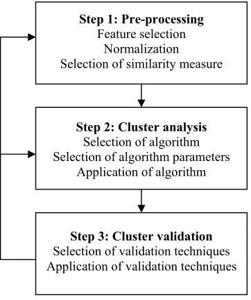
usingclustering techniques. A cluster analysis can beseen as a three step process as outlined in Figure 1.1 [11]. The same methodology is adopted in this study.

The first step involves a number of data transformations including feature selection, normalization and the choice of a distance function, to ensure that related data items cluster together in the data space. When the data set is a set of vectors, as is the case with datasets considered in this study, it is often effective to linearly scale each attribute to zero mean and unit variance, and then apply the Gaussian radial basis function kernel or polynomial kernel [12]. The main advantage of this normalization is to avoid attributes in larger numeric ranges dominating those in smaller ranges. More advanced methods for kernel normalization are described in [13].

The second step consists of the selection, parameterization and application of one or several clustering methods. The resulting partitionings are evaluated in the third step using cluster-validation techniques. Cluster-validation techniques have the potential toprovide an analytical assessment of the amountand type of structure captured by a partitioning, and shouldtherefore be a key toolin the interpretation of clusteringresults [11].

The procedure of evaluating clustering results is known as cluster validity.

Cluster validity methods may assist users in choosing clustering results independently from the clustering algorithms, the parameters and the number of clusters. In general there are three approaches to cluster validity: external, internal

and relative criteria. For some datasets in our experiments reported here, we have

Figure 1.1 The three main steps involved in a cluster analysis: Preprocessing, cluster analysis, cluster validation

Step 1: Pre-processing

Feature selection Normalization Selection of similarity measure

Step 2: Cluster analysis

Selection of algorithm Selection of algorithm parameters

Application of algorithm

Step 3: Cluster validation

CHAPTER 2

A WEIGHTED FUZZY KERNEL BASED METHOD INCORPORATING LOCAL APPROXIMATION FOR CLUSTERING MICROARRAY DATA

Abstract

Data clustering analysis has been extensively applied to extract information from microarray gene expression data. However, finding good quality clusters in gene expression data is more challenging because of its peculiar characteristics such as non-linear separability, outliers, high-dimensionality, and diverse structures. Therefore, this study aims at combining kernel methods, capable of both handling the high dimensionality and discovering nonlinear relationships in the data, with the approximate reasoning offered by fuzzy approach. To this end, a robust Weighted Kernel Fuzzy C-Means incorporating local approximation (WKFCM) is presented. In WKFCM, fuzzy membership of each object is approximated from the memberships of its neighboring objects. It brings in the synergy of partitioning and density based clustering approaches and provides a substantial improvement in the analysis of the data. Comparative analysis with K-means, hierarchical, fuzzy C-means and fuzzy self-organizing maps showed that, although different types of datasets are better partitioned by different algorithms, WKFCM displays the best overall performance, and has the ability to capture nonlinear relationships and non-globular clusters, and identify cluster outliers.

Keywords: Clustering; Kernel methods; Pattern recognition; microarray data analysis;

The task of clustering genes into functionally-similar clusters using expression data rests on the assumption that genes of similar function share similar expression profiles across various experimental conditions. Clustering algorithms have proved useful to help group together genes with similar functions based on gene expression profiles under various conditions or across different tissue samples [14-17]. Such partitioning can facilitate data visualization and interpretation, and it can be exploited to gain insight into the transcriptional regulation networks underlying a biological process of interest. By expanding functional families of genes with known function together with poorly characterized or novel genes may help understand the functions of many genes which are not explored yet.

Since the work of Eisen et al. [17] clustering methods have become a key

step in microarray data analysis. Various clustering algorithms have been applied in the cluster analysis of genes, including HAC (hierarchical agglomerative clustering) [17], SOM (self-organizing maps) [18], CLIFF (Clustering via Iterative Feature Filtering) [19], and algorithms based on mixture models [20], neural networks [21], simulated annealing [22], and PCA (principle components analysis) [23]. There are also many works in co-clustering gene expression matrix, i.e., clustering genes and samples at the same time [24, 25].

However, microarray datasets tend to have very diverse structures due to the complex nature of biological systems. Because of this, none of the existing clustering algorithms perform significantly better than the others when tested across various datasets [11, 14, 16, 26, 27]. Popular algorithms, such as K-Means, hierarchical

widely used clustering algorithm and has become a de facto standard for visualization of expression data, although it has been described to suffer from a number of limitations mostly deriving from the local decision making scheme for constructing clusters that joins the two closest genes or clusters without considering the data as a whole, and it is likely to be a poor choice for further analysis of the resulting clusters [16, 18, 30, 31]. But genes on any given array are not isolated entities: the expression level of a specific gene should affect, or share information with, its biological neighbors. It suggests that Microarray datasets represent the collective behavior of a population best studied jointly; and many current statistical techniques ignore this [32]. In addition, handling of outliers in microarray data is extremely important as one outlier can yield misleading results [14].

More recently, fuzzy clustering approaches have been considered because they may assign one gene to multiple clusters (fuzzy assignment), which may allow capturing genes involved in multiple biological processes. Fuzzy C-Means (FCM) associates each object with every cluster based on the relative distances between the object and the cluster centroids [33, 34]. During the last few years, a number of variants of FCM have been proposed including a variant that incorporates PCA and hierarchical clustering [35], FuzzySOM [36], and Fuzzy J-Means that applies variable neighborhood searching to avoid local minima [37]. However, these FCM based clustering approaches lack the ability to capture non-linear relationships [29]. Some of the fuzzy clustering approaches are based on Gaussian Mixture Models (GMM) [20, 38], which assume the dataset to be generated by a mixture of Gaussian distributions with certain probability. But, the expression data do not always satisfy the basic Gaussian Mixture assumption even after carrying out various transformations aimed at improving the normality of the data distributions [20].

approximation based on the influence of the neighboring objects with the kernel fuzzy approach. It brings in the synergy of partitioning and density based clustering approaches and provides a substantial improvement in the analysis of the target data.

This paper is organized as follows. In the next section, it is briefly pointed out how kernel-based methods can be useful for clustering non-linearly separable and high-dimensional data. In section 3, the proposed algorithm–a Weighted Kernel Fuzzy C-Means incorporating local approximation (WKFCM)–is presented which can be useful for handling of non-linear separability, noise, and outliers in the data. Experimental settings, including evaluation measures, datasets and parameters used, are given in section 4. In section 5, comparative evaluation of WKFCM’s performance on microarray data is given. Finally the paper concludes in section 6.

2. Kernel Methods and Clustering in Feature Space

Over the last decade, estimation and learning methods utilizing positive definite or Mercer kernels have become rather popular, particularly in machine learning. Since these methods have a stronger mathematical slant than earlier machine learning methods (e.g., neural networks), the statistics and mathematics communities have also significant interest in these methods [1]. Among these methods, Support Vector Machines (SVM) is being widely applied in the machine learning community since it often shows better performance than other learning algorithms. A distinctive feature of SVM is the use of Mercer kernels[2] to perform the inner product (kernel trick). The great success of SVM has led to the

development of a new branch of machine learning, Kernel Methods, i.e. the

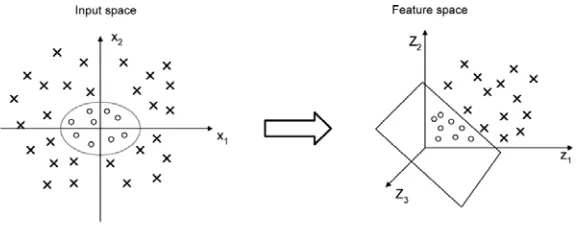
The fundamental idea of the kernel methods is to first transform the original low-dimensional inner-product input space into a higher dimensional feature space through some nonlinear mapping where complex nonlinear problems in the original low-dimensional space can more likely be linearly treated and solved in the transformed space. In the higher dimensional space, data points are spread out, and a linear separating hyperplane may be found. This concept is based on Cover’s theorem on the separability of patterns. According to the Cover’s theorem, an input space made up of nonlinearly separable patterns may be transformed into a feature space where the patterns are linearly separable with high probability, provided the transformation is nonlinear and the dimensionality of the feature space is high enough [5]. However, usually such mapping into high-dimensional feature space will undoubtedly lead to an exponential increase of computational time. Fortunately, adopting kernel functions to substitute an inner product in the original space, which exactly corresponds to mapping the space into higher-dimensional feature space, is a favorable option. Therefore, the inner product form leads us to applying the kernel methods to cluster complex data [6, 7].

Figure 1 illustrates that the two classes in input space may not be separated by a linear separating hyperplane.However, when the two classes are mapped by a nonlinear transformation function, a linear separating hyperplane can be found in the higher dimensional feature space. Let a nonlinear transformation function φ maps the data into a higher dimensional space. Suppose there exists a function κ, called a kernel function, such that,

( , )x x_{i j} =φ( ) ( ).x_i ⋅φ x_j

κ ₍₁₎

Figure 1 Mapping nonlinear data to a higher dimensional feature space where a linear separating hyperplane can be found. When mapped into a feature space via the

non-linear map

_{( ) (}

₎

(

[ ] [ ]

[ ] [ ]

)

1, ,2 3 1 , 2 , 2 1 2

z z z x x x x

φ x = =

The standard “sum-of-squares” (such as Euclidean distance measure) based methods of partitioning (such as K-means, FCM) have proved to be effective for

datasets having ellipsoidal cluster structures [8]. A disadvantage to these methods is that clusters can only be separated by a hyperplane. If the separation boundaries between clusters are nonlinear, for instance non-Euclidean structures in the data such as nonspherical shape clusters, then these methods fail. An attractive approach to solving this problem is to adopt the strategy of nonlinearly transforming the data into a high-dimensional feature space and then performing the clustering within this feature space. To allow non-linear separators, kernel FCM (described in the next section) first uses a function φ to map data points to a higher-dimensional feature space, and then applies FCM in this feature space. Linear separators in the feature space correspond to nonlinear separators in the input space [4]. However, as the feature space may be of high and possibly infinite dimension, then directly working with the transformed variables is an unrealistic option. However, as mentioned above, it is unnecessary to work directly with the transformed variables. It is the inner-products between points which are used and these can be computed using a kernel function in the original data space [2, 4]. This observation provides for a tractable means of working in the possibly infinite feature spaces.

Table 1: Examples of popular kernel functions

Sigmoid Kernel _{( , ) tanh( , )}

i j = γ× i j +β

x x x x

κ γ and β are user defined

values

Polynomial Kernel ( , ) , d

i j =< i j >

x x x x

κ _{d is a positive integer}

Gaussian Kernel (Radial Basis Function)

2 ₂

( , ) exp(x xi j = − xi−xj / 2σ )

κ _{σ is a user defined value}

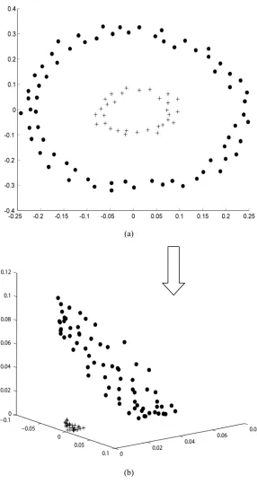
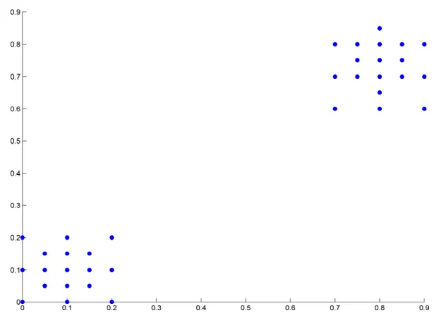
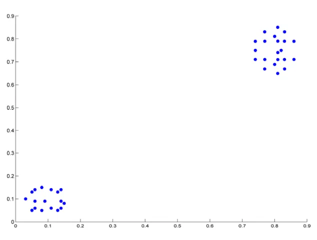
We use a small example to motivate the kernel idea. Suppose we want to cluster the 100 two-dimensional points in Figure 2(a) into 2 clusters such that points on the inner circle are in one cluster and the remaining points are in the other. None of the K-Means or the Fuzzy C-Means can generate the clustering that we want to see

because they only discover clusters that are linearly separable.

Take the K-Means algorithm as an example. To decide whether x belongs to

cluster V1 or V2, we compare distances ||x − v1|| and ||x − v2||. So all the points that

are equally far from v1 and v2 satisfy the equation

||x − v1|| = ||x − v2||,

i.e., xT _(v

1− v2) + (||v2||2− ||v1||2) / 2 = 0,

which describes a hyperplane.

However, if we map the points into three-dimensional space using

2 2

1 1 2 2

( ) [ , 2 , ]T

x x x x

φ x = (2)

Though mapping points to a higher dimensional space, called kernel space or feature space, enables a simple algorithm like the K-Means algorithm to handle

non-linearly separable clusters, computing

φ

space has high dimensionality. However, if an algorithm only depends on the data through inner products, xT _{z, in the original space, then after the mapping it will only}

depend on ( ) ( )φ _x Tφ _{z . Suppose we are given a kernel function κ (x, z), such that}

( , ) = ( ) ( )_{x z} φ _x Tφ _z

κ

then we will not need to know φor

φ

For the mapping function φ in (2), the corresponding kernel function is

2

( , ) = (_{x z x z}T )

κ , a degree 2 polynomial kernel, since

( , ) _{x z} = φ( ) (_x Tφ _z)

κ

2 2 2 2

1 1 2 1 2 2 1 2 2 2

x z x x z z x z

= + +

2 2

1 1 2 2

( ) ( T )

x z x z

= + = x z

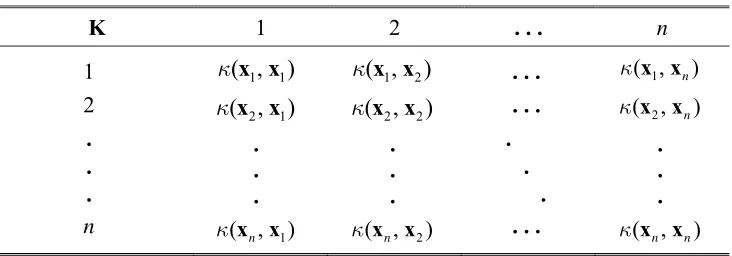
For a given set {x1, x2, ..., xn}, matrix K, where Kst =κ (xs, zt), 1 ≤s, t ≤n, is called a

kernel matrix. Since Κ=[ ( ),..., ( )] [ ( ),..., ( )]φ x₁ φ x_n T φ x₁ φ x_n is the Gram matrix1 of the

images in the feature space; it is a symmetric, positive semidefinite matrix, and since

it specifies the inner products between all pairs of points x , it completely

determines the relative positions of those points in the embedding space. On the other hand, if a given symmetric matrix K is positive semi-definite, we can compute the Cholesky decomposition

K=RT _R,

(a)

(b)

Figure 2 100 points distributed on two concentric circles:

Table 2: Kernel matrix displays

K 1 2 . . . n

1 2 . . . n 1 1 ( , )x x κ

2 1 ( , )x x κ

. . .

1

( , )x x_n κ

1 2 ( , )x x κ

2 2 ( , )x x κ

. . .

2

( , )x x_n κ . . . . . . . . . . . . 1

( , )x x_n κ

2

( , )x x_n κ

. . . ( , )x x_{n n} κ

where the symbol K in the top left corner indicates that the table represents a kernel matrix.

Definition: Gram matrix

Given a set of vectors, S= {x1, x2, ..., xn}, the Gram matrix is defined as the n × n matrix G whose entries are G_ij= x x_i, _j . If we are using a kernel function κ to

evaluate the inner products in a feature space with feature map φ, the associated

Gram matrix has entries

( ), ( ) ( , )

ij= φ i φ j = i j

G x x κx x

In this case the matrix is often referred to as the kernel matrix. We will use a

standard notation for displaying kernel matrices as shown in Table 2, where the symbol K in the top left corner indicates that the table represents a kernel matrix.

The Gram matrix plays an important role in some learning algorithms. The matrix is symmetric since G_ij=G_ji, that is _GT _{=G. Furthermore, it contains all the}

information needed to compute the pairwise distances within the dataset as shown above. This also reinforces the view that the kernel matrix is the central data type of kernel-based algorithms.

_______________________________________

3. Weighted Kernel Fuzzy C-Means (WKFCM) incorporating local approximation

Clustering has received a significant amount of renewed attention with the advent of nonlinear clustering methods based on kernels as it provides a common means of identifying structure in complex data [6, 7, 9, 10, 40].

3.1 Extraction of Local Structure Information

Firstly the local structure information of the data is extracted. To this end, similarities between each pair of objects are calculated (a kernel function is used for measuring similarities, as described below), and the nearest neighbors are identified. The similarity measures between each object and its nearest neighbors are used to estimate the density around that object and to calculate a set of weights for local approximation in the next step. The set of densities forms a rough estimation of the distribution of the dataset, and the resulting values are also used in this step to identify possible cluster outliers.

The K-nearest neighbors (KNN) for each gene are defined as k genes with the highest similarity according to a given similarity measure (kernel similarity measure). The weights defining how much each neighbor will contribute to the approximation of the membership of the object (say, objecti) are calculated as Wij, as shown in Figure 3, with the following relation:

( )

1

ij j KNN i

w ∈

=

∑

Figure 3 Steps for extracting local structure information: (a) Assign neighbors to each data point xi by using the k nearest neighbors. (b) Compute the weights wij that best linearly approximate xi from its neighbors, using the kernel similarity

from the similarities sij between that gene (genei) and its nearest neighbors. The only requirement for a definition of weights is that, the neighbors that have higher similarities must get higher weights. The simplest one we use is:

( )

( )

( , ) ( , )

ij i j

ij

ij i j

j KNN i

j KNN i s w s ∈ ∈ = =

∑

∑

κ . (4)

In other words, the data to be fed to the main iterative procedure for clustering (described in the next subsection) becomes,

( )

i ij j

j KNN i w ∈

=

∑

x x , ₍₅₎

The distance measure is transformed into similarity measure using kernel based transformation to highlight relative proximities of the objects. As the elements of the kernel matrix represent similarities between the respective objects, following the above reasoning, the weights for individual objects can be defined as:

( )

( , )i j j KNN i

i NN w K ∈ =

∑

, (6)

where KNN is the number of nearest neighbors.

The values of the weights for respective objects indicate the relative density around the objects or local density of the objects. The densely populated objects will get higher weights while the outliers and noise points will get lower weights. The first step is the extraction of local structure information and identification of cluster core objects (CCOs); in other words, starting cluster centroids or seed objects. In this step, the similarity (proximity) between each object and its K-nearest neighbors is

number of number of K-nearest neighbors (KNN), the less number of CCOs will be identified, resulting in the less number of generated clusters.

To define possible cluster outliers, a density threshold can be applied so that objects with a density below the threshold are defined as possible outliers (objects with atypical behavior). In addition, this step adds features of the density based clustering approach to the partitioning based clustering approach. In a sense, this local approximation acts as a regularizer and biases the solution toward piecewise-homogeneous labeling. As it can be observed in Figures 6 and 7 that after applying local approximation, the boundary points are shifted towards their cluster centroids; it results in arrangement of clouds of points smoother at the boundaries. To define outliers, if the outliers are expected in the data, we used the following threshold on densities (or weights of individual objects, i.e., weights written with single subscript; whereas the weights written with double subscript represent interconnecting weights):

= 2 (7)

where stands for mean density and stands for standard deviation of the densities.

This approach of incorporating local approximation brings in the following advantages: 1) It gives the estimation of the number of clusters present in the data by identifying cluster core objects (CCOs) which have higher density as compared to their neighboring objects; 2) the iterative procedure of the algorithm starts with the probable cluster centroids (CCOs); it results in fast convergence (less number of iterations) to a global solution; 3) by approximating data points based on the values of their nearest neighbors, the clusters of relevant points become even more compact, whereas the outliers or noise points are less affected (due to RBF kernel function), thus rendering them easy to get treated; it also helps in fast convergence of the algorithm (in less number of iterations) as the iterative procedure converges fast on compact and well separated data.

Figure 4 An example dataset (simulated Data-1) consisting of two clusters.

Figure 5 Data objects are used to calculate for each object a density value

(a)

(b)

3.2 Approximation of Fuzzy Membership

Mathematically, the standard FCM objective function of partitioning a dataset

1 2

{ , ,..., }_n

X = x x x with N

i∈

x (i.e., in N dimensional space) into c clusters,

represented as C={ ,C C_{1 2},..., }C_c , is given by

2

1 1

c n m

m ik i k

k i

J u

= =

=

∑∑

where ⋅ stands for the Euclidean norm. Equivalently, (8) can, in an inner or scalar

product form, be rewritten as

1 1

( 2 )

c n

m T T T

m ik i i i k k k k i

J u

= =

=

∑∑

where V ={ ,v v_{1 2},..., }v_c with N k∈

v are the centroids or prototypes of the clusters

1, 2,..., c

C C C ; T denotes matrix transpose; the parameter m is a weighting exponent on

each fuzzy membership and the array U=[uik] is a fuzzy partition matrix satisfying

[ ]

1 1

0,1 c 1, and 0 n ,

ik ik ik

k i

U u u i u n k

= =

⎧ ⎫

=_⎨ ∈ = ∀ < < ∀ _⎬

⎩

∑

∑

where uikdenotes the membership degree of the ith pattern belonging to the kth cluster. Or,

[ ]

11 12 1

21 22 2

1 2

c c ik

n n nc

u u u

u u u

u

u u u

⎡ ⎤ ⎢ ⎥ ⎢ ⎥ = =_{⎢ ⎥} ⎢ ⎥ ⎣ ⎦ U .

And, m∈ ∞[1, )

is a weighting exponent that controls the membership degree uik of each data point xi to the cluster Ck. As m→1, J1 produces a hard partition where uik ∈ {0,1}. As m approaches infinity, J∞ produces a maximum fuzzy partition where uik = 1/c. This fuzzy c-means-type approach has advantages of differentiating how closely a gene

because it makes soft decisions in each iteration through the use of membership functions.

With the above formulations, we are now in a position to construct the kernelized version of the FCM algorithm and modify its objective function with the mapping

φ

2

1 1

( ) ( )

c n m

m ik i k

k i

J u φ φ

= =

=

∑∑

Now, through the kernel substitution, we have

2

( )_i ( )_k ( ) ( ) 2 ( ) ( )_{i i i k} ( ) ( )_{k k}

φ

φ

φ

φ

φ

φ

φ

φ

2

( )_i ( )_k ( , )_{i i} ( ,_{k k}) 2 ( ,_{i k})

φ

φ

where ( , )κ x xi s =Kis=φ( ) ( )xi ⋅φ xs is a user defined mercer kernel function, which

can be used to represent a dot product in the high dimensional feature space. If the Gaussian radial basis function (RBF) is adopted, viz.

(

)

2

2

( , ) exp i s

i s Kis _σ −

= = − x x

x x

κ . ₍₁₃₎

Then, in this case, ( , )κ x x_{i i} =K_ii =1, so (11) can be simplified as

1 1

2 c n m(1 ( , ))

m ik i k

k i

J u

= =

=

∑∑

3.2.1 Cluster Prototype Updating

In order to minimize (14) with respect to vk, we take the derivative of Jmwith respect to vk, and set the result to zero; so we have

2 1

2

( , ) ( ) 0 n

m m

ik i k i k i

k

J

u

v

σ

∂ _{= − − =}

∂

∑

1 1 ( , ) ( , ) n m

ik i k i i

k n m

ik i k i u u = = =

∑

∑

x v x v

x v κ

κ

,

or, 1

1

( , )

( , ) n

m

ik i k i i

k n m

ik i k i u u = = =

∑

∑

x v x v

x v κ

κ

. (16)

3.2.2 Membership Evaluation

To optimize (14) with respect to uik, we can obtain the following Lagrange

function without constraint,

1 1 1 1

2 c n m(1 ( , )) n c 1

m ik i k ik

k i i k

J u u

= = = =

⎛ ⎞

= − − λ_⎜ − _⎟

⎝ ⎠

∑∑

∑ ∑

where λ is the Lagrange coefficient. Rewrite (17) as follows:

1 1 1 1

2 c n m(1 ( , )) n c 1

m ik i k ik

k i i k

J u u

= = = =

⎛ ⎞

= − − λ_⎜ − _⎟

⎝ ⎠

∑∑

∑ ∑

where (1−κ( ,x v_{i k})) is a weighted similarity measure in the kernel space.

Taking the derivative of Jm with respect to uikand setting the result to zero, we have,

1

2 m (1 ( , )) 0

m

ik i k ik J mu u − ∂ = − − λ =

∂ κ x v . (19)

Solving for uikwe have

1 1

(1 ( , ))

m

ik

i i k

u

mw

−

⎛ λ ⎞

= ⎜ ₋ ⎟

⎝ κ x v ⎠ . (20)

Considering the constraint u_ik∈[0,1] and

1 1 c ik k u = =

∑

1 1

1

1

(1 ( , ))

m

c

k mwi i k

− = ⎛ λ ⎞ = ⎜ ₋ ⎟ ⎝ ⎠

∑

or, 1 1 1 1 1

(1 ( , ))

m

m c

k i k

m m − − = λ = ⎛ _{⎛ ⎞} ⎞ ⎜ _{⎜ ⎟} ⎟ ⎜ _⎝ − _⎠ ⎟

⎝

∑

. ₍₂₂₎

Substituting it into (20), the zero-gradient condition for the membership estimator can be re-written as

1 1

1 1

1

(1 ( , ))

(1 ( , ))

m m i k ik c i l l u − − = − = −

∑

. (23)

This solution also satisfies the remaining constraints of Equation (10). Therefore, the cluster centroids and membership degrees in (16) and (23) are optimized in each iteration by minimizing the functional Jm .

3.3 Cluster Construction

have one dominant membership value. The objects not assigned to any cluster can be regarded as outliers or noise points. Such points can be screened out from the clusters.

WKFCM can be summarized in the following subsection.

3.4 Algorithm WKFCM

The algorithmic steps of WKFCM are as follows:

Algorithm Weighted Kernel Fuzzy c-Means (WKFCM)

WKFCM (K, [c], KNN)

Input: K: kernel matrix, c: number of clusters (optional), set ε > 0 to a very

small value as a termination criterion, K_NN: number of nearest neighbors of a point,

Output: v1, ..., vc: partitioning of the points

1. Input the dataset X = {x1, x2, ..., xn} with xi∈ N

2. For each object x, compute weights using equation (6),

( )

( ,_{i p})

p KNN i i

NN w

K ∈

=

∑

x x κ

, (6)

and find CCOs (cluster core objects) as initial cluster centroids (for

c clusters: v1, ...,vc ), and identify outliers, if any.

3. Approximate the data based on neighborhood information using the

following relation:

( )

i=

∑

x x

4. Set r = 0; initialize U( )r = ⎣ ⎦⎡u_ik( )r ⎤ of xi belonging to cluster Ck for 1 ≤

k ≤c, 1 ≤i ≤n such that

1

1

c ik k

u =

=

∑

1 ( ) 1 1 ( ) 1 ( 1) 1

(1 ( , ))

(1 ( , ))

r m r

m

r i k

ik c i l l u − − + = − = −

∑

6. Update the centroids ( 1) ( 1) ( 1) ( 1)

1 2

{ , ,..., }

r r r r

c

V + = v + v + v + for 1 ≤i ≤c

using equation (16)

( )

( )

( 1) ( 1) 1

( 1) 1 ( ) ( , ) ( ) ( , ) r r n r m

ik i k i r i

k n

r m

ik i k i u u + + = + = =

∑

∑

x v x

v

x v κ

κ

(16)

7. Stop if the following termination criterion is met:

( 1)r ( )r

V + −V <

ε

(

)

such as max r r , for 1 and1 0.0001

kj kj

v + −v ≤ ≤k c ≤ ≤j N ≤

whereV ={ , ,..., }v v_{1 2} v_c , or, the maximum number of iterations is reached. Otherwise, set r=r+1 and return to step 5.

4. Experimental Settings

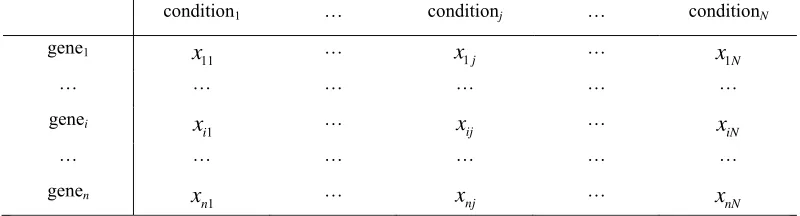
Gene expression data are generated by DNA chips and other microarray techniques. The raw data produced by microarray often come along with noise, missing values and systematic variations [44]. Preprocessing, such as estimation of missing values [45], normalization [46, 47], is needed. After the above preprocessing steps, gene expression data can be represented as a real-valued matrix, in which the entry at row i and column j is the measured expression level of genei under conditionj, as shown in Figure 8.

condition1 … conditionj … conditionN

gene1 _x11 … ₁

j

x … x_1N

… … … …

genei

1

i

x … x_ij … x_iN

… … … …

genen

1

n

x … x_nj … x_nN

Figure 8 Gene expression data matrix

4.1 Evaluation Measures for Clustering

Evaluating clustering results is a tricky business. However, in situations where data points are already categorized (labelled), we can compare the clusters with the “true” class labels and calculate classification rate. To evaluate the goodness of the clustering produced by the algorithms on the test data without true class labels, two validity measures were used in this study: the Figures of Merit (FOM), and the Davies-Bouldin Index (DBI).

4.1.1 Classification accuracy

To compare the clustering results of different algorithms on the data for which class labels are known, classification accuracy or classification rate is defined as:

Number of correctly classified points

Classification accuracy (%) = 100

4.1.2 Figures of Merit

The FOM of Yeung et al. [48] estimates the predictive power of a clustering method based on the jackknife approach. The method measures the root mean square deviation in the left-out condition of the individual gene expression level relative to their within-cluster means. As each condition is used as the validation condition, it calculates the sum of FOMs over all the conditions. Meaningful clusters exhibit less variation in the remaining conditions than clusters formed by random. Thus, a lower value of FOM represents a well-clustered result, representing that a clustering method has high predictive power.

The use of Figures of Merit (FOMs) has been proposed by Yeung et al. [48,

49] to characterize the predictive power of different clustering algorithms. FOM is estimated by removing one experiment at a time from the dataset, clustering genes based on the remaining data, and then measuring the within-cluster similarity of the expression values in the left-out experiment. The principle is that correctly co-clustered genes should retain a similar expression level also in the left-out sample. The assumption (and limit) of this approach is that most samples have correlated gene expression profiles. The most commonly used FOM, referred to as "2-Norm FOM" [48], measures the within-cluster similarity as root mean square deviation from the cluster mean in the left-out condition. An aggregated FOM is obtained by summing up all the FOMs of all left-out experiments and is used to compare the performance of different clustering algorithms (the lower the FOM, the better the predictive power of a clustering algorithm). Since it is a rather novel measure, a formal definition is provided below.

For a given dataset, let R denotes the raw data matrix. Assume that R has

dimension n × N, i.e., each row corresponds to a gene and each column corresponds

to an experimental condition. Assume that a clustering algorithm is given the raw matrix R with column e excluded. Assume also that, with that reduced dataset, the

algorithm produces c clusters R1, ..., Rc. Let r( , )g e be the expression level of gene g

(

)

1 FOM( , )

k k i

c

g e i e i g R

e c r m

n = ∈

=

∑ ∑

Notice that FOM(e,c) is essentially a root mean square deviation. The aggregate

2-Norm FOM for c clusters is then:

1

FOM( ) N FOM( , )

e

c e c

=

=

∑

Both formulae (24) and (25) can be used to measure the predictive power of an algorithm. The first gives us more flexibility, since we can pick any condition, while the second gives us a total estimate over all conditions. Moreover, since the experimental studies conducted by Yeung et al. [48, 49] show that FOM(c) behaves

as a decreasing function of c, an adjustment factor has been introduced to properly

compare clustering solutions with different numbers of clusters. A theoretical analysis by Yeung et al. [48] provides the following adjustment factor:

n c

n

−

. (26)

When (24) is divided by (26), (24) and (25) are referred to as adjusted FOMs. We

use the adjusted aggregate 2-Norm FOM for our experiments, and we refer to it simply as 2-Norm FOM.

4.1.3 Davies-Bouldin Index (DBI)

The Davies-Bouldin Index (DBI) aims at identifying sets of clusters that are compact and well separated [50]. Small values of DBI correspond to clusters that are compact, and whose centres are far away from each other. For any partition

1 2 ...

: _c

1

( ) ( )

1

( ) max

( , )

c

i j

i j

i i j

C C

DBI W

c ₌ ≠ δ C C

⎧Δ + Δ ⎫

⎪ ⎪

= ⎨ ⎬

⎪ ⎪

⎩ ⎭

∑

here δ( ,C Ci j) defines the inter-cluster distance between the clusters Ci and Cj; ( )C_i

Δ represents the intracluster distance of cluster Ci , and c is the number of clusters of partition W.

Different methods may be used to calculate intercluster and intracluster distances [11]. Mathematical definitions of the intercluster and intracluster distances used in our experiments are given in the following subsections. For details, please see [11].

4.1.3.1 Intercluster Distances

Six intercluster distances may be used for the calculation of the Davies-Bouldin validity indices. The single linkage distance defines the closest distance

between two samples belonging to two different clusters. The complete linkage

distance represents the distance between the most remote samples belonging to two different clusters. The average linkage distance defines the average distance between

all of the samples belonging to two different clusters. The centroid linkage distance

reflects the distance between the centres of two clusters. The average of centroids linkage represents the distance between the centre of a cluster and all of samples

belonging to a different cluster. Hausdorff metrics are based on the discovery of a

maximal distance from samples of one cluster to the nearest sample of another cluster. In this study, average linkage distance is used which is defined below:

1 1 2 2

1 2 1 2

, 1 2

1

( , ) ( , )

x C x C

C C d x x

C C

δ

∈ ∈

=

∑

where C₁ and C ₂ are clusters from partition W; d x x( , )_{1 2} defines the distance

between any two samples, x₁ and x₂, belonging to C₁ and C , ₂ respectively; C1 and

2

4.1.3.2 Intracluster Distances

Three intracluster distances may be used to calculate the Davies-Bouldin validity indices. The complete diameter distance represents the distance between the

most remote samples belonging to the same cluster. The average diameter distance

defines the average distance between all of the samples belonging to the same cluster. The centroid diameter distance reflects the double average distance between all of

the samples and the cluster's centre. In this study, average diameter distance is used

which is defined below:

1 2

1 2

1 2 ,

1

( ) ( , )

( 1) i

i

x x C i i

x x

C d x x

C C ∈

≠

Δ =

−

∑

where C_i is a cluster from partition W; d x x( , )_{1 2} defines the distance between any

two samples, x₁ and x₂, belonging to C_i; C_i represents the number of samples included in cluster Ci.

4.2 Microarray Datasets and Analysis Parameters

To assess the performance of WKFCM and compare it with other popular algorithms, such as K-Means, Hierarchical clustering [35], Fuzzy C-means (FCM)

[33], Fuzzy SOM (FSOM) [36], we used three different datasets: (i) Peripheral Blood Monocytes (PBM) dataset [26], (ii) yeast cell cycle (YCC) expression dataset [51], and (iii) hypoxia response (HR) dataset [15]. Further details on the datasets and parameters used are provided in the following subsections.

4.2.1 Peripheral Blood Monocytes (PBM) dataset

contains 2329 cDNAs with a fingerprint of 139 oligos (performed with 139 different Oligonucleotide probes) derived from 18 genes. The spotted cDNAs derived from the same gene should display a similar profile of hybridization to the 139 probes and therefore be clustered together. Since FOM analysis is too time demanding, Di Gesu

et al. [26] reduced the dataset (PBM) to contain 235 cDNAs. So, the dataset used for

our experiments is also a 235×139 data matrix.

4.2.2 Yeast Cell Cycle (YCC) Data

This yeast cell cycle data is a part of the studies conducted by Spellman et al.

[51]. The complete dataset contains about 6178 genes under 76 experimental conditions. The reduced yeast cell cycle (YCC) dataset is a subset of the original YCC dataset selected by Yeung et al. [48, 49] for FOM analysis and is composed of

698 genes under 72 experimental conditions. We also used the same dataset for our experiments.

4.2.3 Hypoxia Response (HR) Data

The hypoxia response (HR) dataset has been used by Chi et al. [15] to

4.2.4 Parameters

The following parameters were used for all the datasets: cosine correlation was used as a distance metric for all other methods except WKFCM; un-weighted pair-group average linkage for hierarchical clustering; 600 as a maximum number of iterations and ε=0.0001 as the converging criteria for all methods except hierarchical clustering. Clusters with a large range of cluster numbers were generated for the

comparison. The fuzziness parameter m=1.2 was used for FCM, FSOM and

WKFCM. In addition, for WKFCM, we used Gaussian RBF kernel with KNN=4.

5. Evaluation of WKFCM

5.1 Experimentation on Simulated Data-2

The simulated dataset (Data-2) is a two-dimensional set formed by 111 points (86 points in one cluster, 19 points in the other cluster, 6 outliers). The Data-2 is

shown in Figure 9. For comparison, we tried K-Means SOM [28] and Neural Gas

Figure 9 A simulated dataset (Data-2); 86 points in one cluster, 19 points in the other cluster, 6 outliers. Both of the clusters are represented with a different gray level. Filled disks indicate the data points belonging to respective clusters. Circles represent outliers.

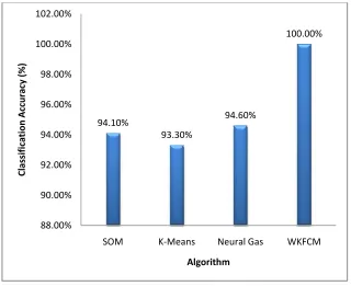
Figure 10 Average WKFCM, SOM, Neural Gas and K-Means performances on simulated Data-2; 111 patterns, 2 features, 2 classes plus outliers. The results have been obtained using ten different runs for each algorithm.

94.10%

93.30%

94.60%

100.00%

88.00% 90.00% 92.00% 94.00% 96.00% 98.00% 100.00% 102.00%

SOM K‐Means Neural Gas WKFCM

Cl

assi

fica

ti

on

Accur

acy

(%)

5.2 Experimentation on IRIS Data

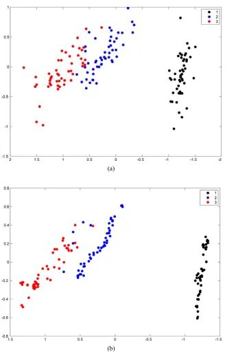
IRIS dataset (IRIS dataset can be downloaded from the address: http://www.ics.uci.edu/~mlearn/databases/IRIS/) is the most famous real data benchmark in Machine Learning. IRIS dataset was proposed by Fisher in 1936 [54]. This dataset is formed by 150 points that belong to three different classes. One class is linearly separable from the other two, but the other two are not linearly separable from each other. Since the dimension of IRIS data is 4, IRIS data is usually represented by projecting the data along their principal components. IRIS data projected along the two components is shown in Figures 7(a). We tried WKFCM, K

-Means, Neural Gas and SOM on IRIS data using three centers, one center for each

class. The results using SOM, Neural Gas, K-Means and WKFCM are shown in

Figure 11.

Figure 11 Average WKFCM, SOM, Neural Gas and K-Means performances on IRIS data; 150 patterns, 4 features, 3 classes. The results have been obtained using thirty different runs for each algorithm.

81%

89%

91.70%

94.70%

70% 75% 80% 85% 90% 95% 100%

SOM K‐Means Neural Gas WKFCM

Cl

assi

fica

ti

on

Accur

acy

(%)

5.3.3 Experimentation on Microarray Data

The clustering performance was firstly evaluated using a Figure Of Merit (FOM), 2-Norm FOM. 2-Norm FOM analysis (as shown in Figures 12, 13 and 14) indicated that no clustering algorithm was the best on all the datasets, with WKFCM, FCM and FSOM being the best, respectively, on the reduced PBM, HR and YCC data.

Whereas, according to the Davies-Bouldin Index analysis (as shown in Figures 15, 16 and 17), WKFCM emerged as the best algorithm on all the three datasets. As WKFCM may generate non-globular clusters with more heterogeneous size distribution, its results for the DBI analysis proved to be the best. Whereas for the FOM analysis, FOM is calculated by averaging the deviations in the left-out condition not cluster by cluster, but by averaging over the whole dataset. Therefore, large clusters with high internal variability have a higher weight in FOM calculation than small, compact clusters.

40 45 50 55 60 65 70 75

0 5 10 15 20 25 30 35

2-No

rm

F

O

M

Number of Clusters

FCM FSOM KMeans Hierarch. WKFCM

50 60 70 80 90 100 110

0 10 20 30 40 50 60 70 80

2-N

o

rm

F

O

M

Number of Clusters

FCM FSOM KMeans Hierarch. WKFCM

Figure 13 Clustering validation and comparison by 2-Norm FOM–lower values of 2-Norm FOM are better. 2-Norm FOM on the reduced hypoxia response (HR) dataset.

47 52 57 62

0 10 20 30 40 50 60

2-N

o

rm

F

O

M

Number of Clusters

FCM FSOM Kmeans Hierarch. WKFCM

0 0.1 0.2 0.3 0.4 0.5 0.6 0.7 0.8

0 5 10 15 20 25 30 35

D a v ie s -B oul di n I nde x

Number of Clusters

FCM FSOM KMeans Hierarch. WKFCM

Figure 15 Clustering validation and comparison by Davies-Bouldin Index–lower values of DB Index are better. DB Index on the reduced peripheral blood monocyte (PBM) dataset. 0.25 0.3 0.35 0.4 0.45 0.5 0.55 0.6

0 20 40 60 80 100

D a v ie s -B oul di n I nde x

Number of Clusters

FCM FSOM KMeans Hierarch. WKFCM

0.5 0.55 0.6 0.65 0.7 0.75 0.8 0.85 0.9

0 10 20 30 40 50 60 70 80

D

a

v

ie

s

-B

oul

di

n I

nde

x

Number of Clusters

FCM FSOM KMeans Hierarch. WKFCM

Figure 17 Clustering validation and comparison by Davies-Bouldin Index–lower values of DB Index are better. DB Index on the reduced yeast cell cycle (YCC) dataset.

Table 3: Ranking of each clustering algorithm across all comparative validation cases (lower value of rank stands for better performance)

Dataset (reduced)

Validation case

WKFCM Hierarch. K-Means FSOM FCM

PBM 2-Norm FOM

DB Index 1 2 5 1 4 5 2 4 3 3

HR 2-Norm FOM

DB Index 4 1 5 4 3 5 2 2 1 3

YCC 2-Norm FOM

DB Index 4 1 5 5 3 4 1 2 2 3

The possible applications of WKFCM can be extended to other than gene expression datasets. WKFCM can be applied to any dataset if a neighborhood can be defined for each object. In comparison with the other clustering algorithms, WKFCM is more robust with respect to outliers and noise, since it has a mechanism that permits discarding outliers and noise. However, one main quality of WKFCM lies in producing nonlinear separation surfaces among data. WKFCM can separate classes of data that are not linearly separable by the other clustering algorithms.

WKFCM’s main limitation is the computation time required by the algorithm. However, the availability of faster machines and low cost of memory encourages the applicability of WKFCM in real world applications.

6. Conclusions

A Kernel based Method, Weighted Kernel Fuzzy C-Means incorporating local approximation (WKFCM), has been presented in this paper. WKFCM is especially suitable for clustering data with fuzzy structures, having nonlinearly separable clusters, such as microarray gene expression data.

solution of real world problems. Future work includes extension of experimental validation to image segmentation.

Acknowledgements

This work was supported in part by the Ministry of Higher Education under Fundamental Research Grant Scheme (Project Number 78096).

CHAPTER 3

CONCLUSIONS

3.1 Introduction

Traditionally, theory and algorithms of machine learning and statistics has been very well developed for the linear case. Linear modeling techniques explicitly assume linear relations between the input and output variables, but in many real-life case studies, the relations are typically observed to be nonlinear. In kernel methods, the implicit kernel induced feature space interpretation allows to extend the linear methods to kernel methods for nonlinear modeling. In this study we have investigated Kernel Methods for Clustering, namely Kernel Methods that do not

require target data.

3.2 Conclusion

In this study, a Weighted Kernel Fuzzy C-Means (WKFCM) has been presented. WKFCM is especially suitable for clustering data with fuzzy structures, such as microarray gene expression data.

combination of advantageous features, some of which are distinctive, like the ability to capture dataset-specific structures by defining neighborhood relations and the subsequent approximation of fuzzy memberships influenced by neighborhood, so that non-globular and non-linear clusters can also be captured and do not get fragmented by the process. In particular, it is the novelty of neighborhood approximation that makes WKFCM distinct from all other clustering approaches. It has the mechanism for defining outlier genes whose expression patterns do not allow reliable assignment to any cluster. Other interesting features are common to fuzzy clustering algorithms, like non-univocal assignment of memberships to genes. Our results also confirm that no clustering strategy is always the best for any data type, which renders the choice between different algorithms.

3.3 Future Work

As WKFCM is not computationally very efficient, therefore a first line of research involves the optimization or efficient implementation of the WKFCM. Another future research line is the development of the specific application oriented kernels, instead of the gaussian one, that can be used in the WKFCM. Another future work could be the extension of WKFCM for clustering incomplete data.

REFERENCES

1. Hofmann, T., B. Schölkopf, and A.J. Smola, Kernel methods in machine

learning. To appear in: Annals of Statistics 2007. 156(2007).

2. Vapnik, V., Statistical Learning Theory. 1998: John Wiley & Sons.

3. Cristianini, N. and J.S. Taylor, An Introduction to Support Vector Machines.

2000: Cambridge Academic Press.

4. Schölkopf, B., A.J. Smola, and K.R. Müller, Nonlinear component analysis as a kernel eigenvalue problem. Neural Computation, 1998. 10(5): p. 1299–

1319.

5. Cover, T.M., Geomeasureal and statistical properties of systems of linear inequalities in pattern recognition. IEEE Transactions on Electronic

Computers, 1965. EC-14(3): p. 326–334.

6. Dhillon, I.S., Y. Guan, and B. Kulis, Weighted Graph Cuts without

Eigenvectors: A Multilevel Approach. IEEE Transactions on Pattern Analysis

and Machine Intelligence, 2007. 29(11): p. 1944–1957.

7. Girolami, M., Mercer kernel based clustering in feature space. IEEE

Transactions on Neural Networks, 2002. 13(3): p. 780–784.

8. Jain, A.K., M.N. Murty, and P.J. Flynn, Data clustering: a review. ACM

Computing Surveys, 1999. 31(3): p. 264–323.

9. Camastra, F. and A. Verri, A novel kernel method for clustering. IEEE

Transactions on Pattern Analysis and Machine Intelligence, 2005. 27(5): p. 801–805.

10. Filippone, M., et al., A survey of kernel and spectral methods for clustering.