ABSTRACT
SAYRES JR., JOHN SCOTT. Computational Fluid Dynamics for Pulsejets and Pulsejet Related Technologies. (Under the direction of Dr. William L. Roberts).
The pulsejet is one of the simplest forms of air-breathing propulsion ever developed. They are scalable, light weight, low cost, and fairly efficient at converting fuel to heat and thrust. This research effort focuses on the using mainly computational software to simulate and predict the working nature of the pulsejet.
There is an emphasis on expanding on previous research on 50 cm valved pulsejets and adapting this technology to smaller sizes of 25 cm and 12 cm. The performance of these pulsejets can be improved by the use of an augmenter and in this report there is a large study on how the free stream flight speed affects this performance improvement. Lastly, there is also an effort in modeling valveless pulsejets on the 5 cm to 25 cm scale.
Computational Fluid Dynamics for Pulsejets and Pulsejet Related Technologies.
by
John Scott Sayres, Jr.
A thesis submitted to the Graduate Faculty of North Carolina State University
in partial fulfillment of the requirements for the degree of
Master of Science
Aerospace Engineering
Raleigh, North Carolina 2011
APPROVED BY:
_______________________________ ______________________________ Dr. William L. Roberts Dr. Tarek Echekki
Committee Chair
ii
DEDICATION
iii
BIOGRAPHY
John S. Sayres, Jr. was born in Baltimore, Maryland on November 10, 1986. After spending several years in Maryland he and his family relocated to Greensboro, North Carolina in the fall of 1991. In Greensboro he spent his childhood with an academic fascination in science and math as well as several extracurricular hobbies including
basketball, football, track, videogames, and music. He picked up the electric guitar in 2001 and has played in several local bands with an affinity for hard rock and heavy metal. He graduated from Northwest Guilford High School in May of 2004.
After graduating High School, John immediately enrolled at North Carolina State University majoring in Aerospace Engineering with a minor in Physics. John graduated cum laude with a Bachelor of Science in May of 2009 and followed immediately into the graduate school at NC State under the advising of Dr. William L. Roberts. After completing his
iv
ACKNOWLEDGMENTS
v
TABLE OF CONTENTS
LIST OF FIGURES ... vii
LIST OF TABLES ... ix
CHAPTER 1 - Introduction ... 1
1.1HISTORY ... 1
1.2THEORY AND JET DESIGN ... 4
1.3PREVIOUS RESEARCH ... 8
1.3.1 Experimental Research at NCSU ... 8
1.3.2 Computational Research at NCSU ... 10
1.4GOALS OF THIS PROJECT ... 11
CHAPTER 2 – Computational Setup ... 12
2.1HARDWARE ... 12
2.2SOFTWARE ... 13
2.2.1 Working with ANSYS ... 13
2.2.2 Working with CFX ... 16
CHAPTER 3 – Valveless Pulsejets ... 18
3.1FUEL INJECTION ... 18
3.2VALVELESS 12 CM PULSEJET ... 19
3.3INLET OPTIMIZATION ... 23
3.4U-SHAPED PULSEJETS ... 25
3.4.1 U-Shaped Pulsejet Drag ... 26
3.4.2 U-Shaped Pulsejet Thrust ... 28
vi
4.1FUEL-AIR MIXTURE RATIO EFFECT ... 33
4.2SICKLE VALVE 3-DSIMULATIONS ... 36
CHAPTER 5 – Augmenter Effects ... 39
5.1EFFECT OF FORWARD FLIGHT SPEED ON AUGMENTER PERFORMANCE ... 41
5.1.1 Steady State Aerodynamic Drag ... 43
5.1.2 Augmented 50 cm Pulsejet Thrust in Varying Convective Streams ... 44
CHAPTER 6 – Further Experiments ... 49
6.1WIND TUNNEL TESTING ... 49
6.1.1 Experimental Wind Tunnel ... 49
6.1.2 CFD Wind Tunnel ... 51
6.2COLD FLOW TESTING ... 55
6.2.1 Cold Flow CFD Testing ... 56
CHAPTER 7 - Conclusions ... 61
REFERENCES ... 62
APPENDIX ... 64
vii
LIST OF FIGURES
Figure 1-1: Simple valveless pulsejet in half section view ... 2
Figure 1-2: U-Shaped pulsejet ... 3
Figure 1-3: V-1 “Buzz-Bomb” with Aurgus As 014 pulsejet powerplant ... 4
Figure 1-4: General pulsejet design with flare ... 5
Figure 1-5: p-V diagram for the Humphrey Cycle ... 6
Figure 1-6: Running 25 cm pulsejet ... 9
Figure 2-1: 2-D ANSYS geometry ... 14
Figure 2-2: 3-D ANSYS geometry ... 14
Figure 2-3:CFD Wind Tunnel dimensions ... 15
Figure 2-4: Valved pulsejet with augmenter mesh ... 16
Figure 3-1: Symmetric four hole fuel injector ... 19
Figure 3-2: Valveless 12cm pulsejet with varying combustion chamber to exhaust tube lengths ... 20
Figure 3-3: Varying transition length data plotted with trend line ... 21
Figure 3-4: 25 cm variable inlet valveless pulsejet ... 23
Figure 3-5: 25 cm variable inlet valveless pulsejet thrust with trend line ... 24
Figure 3-6: 31cm U-shaped jets. No aerodynamic cone (top) and with aerodynamic cone (bottom) ... 27
Figure 3-7: 28cm U-shaped jet enclosed in smooth NACA 0012 Airfoil ... 28
viii
Figure 3-9: 25cm U-shaped chamber pressure (top) compared with 31 cm U-shaped chamber
pressure (bottom) ... 30
Figure 4-1: 12 cm 2-D valved pulsejet. Valve location highlighted in red. ... 34
Figure 4-2: Sickle valve with fuel injection points (shown in red) ... 37
Figure 5-1: Running 50cm, valved, pulsejet with augmenter ... 40
Figure 5-2: Augmenter location as prescribed by Fei Zheng ... 40
Figure 5-3: 50 cm valved pulsejet with augmenter half-section view ... 42
Figure 5-4: 50 cm valved pulsejet with augmenter CAD model ... 43
Figure 5-5: Total thrust vs free stream velocity ... 46
Figure 6-1: Wind tunnel with pulsejet on sting and dynamometer ... 50
Figure 6-2: Close up on dynamometer ... 51
Figure 6-3: CFD 6” wind tunnel with 12 cm pulsejet on NACA 0012 sting ... 52
Figure 6-4: Drag versus free stream velocity, computational drag compared with experimental drag ... 54
Figure 6-5: Experimental cold flow testing rig courtesy of Joe Scroggins ... 56
Figure 6-6: CFD cold flow testing device ... 57
ix
LIST OF TABLES
Table 3-1: Varying transition length data ... 22
Table 3-2: Coefficient of drag on the u-shaped jet. ... 27
Table 3-3: U-Shaped pulsejet thrust at various lengths ... 31
Table 4-1: Equivalence ratio performance results ... 35
Table 4-2: Sickle valve performance results at three fuel injection rates ... 38
Table 5-1: Drag on augmenter alone with increasing free stream velocity ... 44
Table 5-2: Performance of 50 cm valved pulsejet with augmenter ... 45
Table 5-3: Thrust measured at the exit of the pulsejet with augmenter ... 47
Table 6-1: Drag and Cd for 12 cm jet on NACA 0012 sting in 6” CFD wind tunnel ... 53
1
CHAPTER 1
- Introduction
Introduction
1.1 History
The pulsejet is one of the simplest forms of propulsion known to man. They are known for having little to no moving parts, scalability, relatively low cost, ease of use, and extremely high noise. Pulsejets at the simplest level work by means of pulsed combustion and were invented in the early 1900s.
2
Figure 1-1: Simple valveless pulsejet in half section view
3
Figure 1-2: U-Shaped pulsejet
4
Figure 1-3: V-1 “Buzz-Bomb” with Aurgus As 014 pulsejet powerplant
Nowadays the pulsejet is widely known as more of a hobby for many “garage
engineers.” Due to the high heat output in noises on the order of 100 dB pulsejets aren’t very practical for commercial propulsion use. But, they still exist in the realms of experimental analysis, and it is off of these many designs that the research at NC State has been based for the past decade. This project will delve into what does and doesn’t work with these designs and how to best improve upon them.
1.2 Theory and Jet Design
The operation of the pulsejet has been fairly well known for nearly a century. Because the jet has few moving parts it is almost completely described by its acoustic properties throughout the jet. There has been a large amount of computational and
5
The main design of any pulsejet consists of three main sections as shown below in Figure 1-4. The inlet is a round tube that serves as the main method of inhaling fresh air into the system on each cycle. It is generally the shortest section of the pulsejet and, thus, also has the smallest cross sectional area. After the inlet there can either be valves, which cyclically restrict mass from flowing back through the inlet, or the jet can operate “valvelesslly” in which there is no restrictor. Next, the inlet leads into the combustion chamber. The combustion chamber generally has the largest cross sectional area and serves as a sort of stagnation zone for the fresh air to mix with injected fuel for combustion. The inlet with the combustion chamber can be thought of as a Helmholtz resonator. The combustion chamber then leads into the exhaust tube, which can be thought of as a simple wave tube. The exhaust tube is generally much longer than the inlet and thus has a slightly bigger cross sectional area, not to exceed that of the combustion chamber. This exhaust tube can also have a flare on the end to help with vortex generation and direction.
6
Pulsejets operate on the Humphrey cycle as shown in Figure 1-5. The four step cycle starts at state 1 with isentropic compression followed by isochoric heat addition, isentropic expansion, and lastly, isobaric heat rejection as it returns to state 1.
Figure 1-5: p-V diagram for the Humphrey Cycle
7
!! = !! 2!
S!
VL!
2!!!! !!!! tan
2!!!!!
c! = 1
These symbols are representative of the following values where i describes the inlet properties and e describes the exhaust tube properties:
f Frequency
c Local Speed of Sound S Cross-Sectional Area L Length
V Combustion Chamber Volume
8
length, desired radius of the exhaust tube, and the ratio of the inlet volume to the combustion chamber volume. Once all of the parameters of the jet are pinned down a model can be created using CAD software.
1.3 Previous Research
1.3.1 Experimental Research at NCSU
9
Figure 1-6: Running 25 cm pulsejet
Michael Schoen found that a jet’s operation is mainly characterized by the relationship between the length of the jet and the kinetics of the fuel as well as the
10
located about a third of the way into the combustion chamber where the fuel should be injected. There have also been studies on the direction of fuel injection which include injecting axially down the centerline or in the radial direction from the centerline out to the combustion chamber walls [9].
Joe Scroggins also participated in understanding how “augmenters” can help increase net thrust on a static jet. Experimentally he found that an augmenter can produce a net increase in thrust by up to a factor of 2 when run statically. Scott Steimnetz performed a fuel study and found that these fuels have varying performance based on their kinetics. A study run concurrently with my project is looking at how heating the fuel can allow a jet to run when it previously would not run on the unheated fuel because the kinetics were not fast enough. This has lead to the selection of Propane as the fuel of choice for jets above 12 centimeters and Hydrogen for smaller jets.
1.3.2 Computational Research at NCSU
11
studied constant volume combustion as well as valved pulsejets. I have conducted experiments on many of these previous areas of research in hopes of expanding our knowledge of these pulsejets.
1.4 Goals of this Project
12
CHAPTER 2
– Computational Setup
Computational Setup
2.1 Hardware
Because this research project has a heavy basis on computational fluid dynamics the majority of the research was done on computers. Three main computational devices were used for this project. While I was learning how to build CFD simulations, early testing was done on the NCSU IBM Blade Center which is powered by a 3.0 GHz Intel Xeon processor. This blade center is known as High Performance Computing, or HPC.
The majority simulations presented in this report were split between two other Dell workstations. One workstation housed a dual quad-core 2.4 GHz Intel Xeon processor and 24 GB of RAM while the second workstation housed a dual quad-core 2.33 GHz Intel Xeon processor 16 GB of RAM. Because these machines each contained eight physical CPUs I was able to run up to eight separate CFD jobs at once. This is beneficial because the run time could vary anywhere from a few hours up to several weeks. For the average pulsejet
13
2.2 Software
The hardware used for all computing was backed up by a variety of strong
commercial engineering packages. The CAD modeling was done using either SolidWorks 2009 or ANSYS 11 Workbench. All of the CFD was done on CFX 11 using its -pre, -solver, and -post functionality. For valved pulsejet simulations the valve dynamics were calculated using a FORTRAN subroutine.
2.2.1 Working with ANSYS
14
Figure 2-1: 2-D ANSYS geometry
15
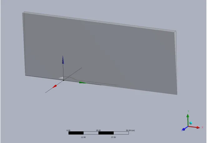
Due to the nature of the simulations being run in a wind tunnel it is necessary to take into account any boundary and wall effects that wouldn’t be seen in free stream conditions. The wind tunnel boundaries are generally created with sufficient distance from the jet that any boundary effects are negligible [6]. This is shown in Figure 2-3 where the boundaries are a fixed distance from the jet based on the jet inlet and outlet sizes.
Figure 2-3:CFD Wind Tunnel dimensions
In this case the dimensions are given as a factor of the di, the inlet diameter, or do, the exhaust tube diameter. These are chosen to reduce any wall effects such as reflected
compression or expansion waves.
After the geometry file is made it is necessary to create a mesh for the solver to calculate all of the flow conditions. This is also done in ANSYS. For 2-D cases a single layer is used for the thickness of the wedge. Inflation is used for all cases to help accurately
16
Figure 2-4: Valved pulsejet with augmenter mesh
A typical 2-D mesh contains around 12,000 mesh cells whereas a 3-D mesh could contain 500,000 to 1,000,000 mesh cells. Once the mesh is created I can then begin to create the definition file to run the simulation in CFX with.
2.2.2 Working with CFX
The mesh file created in ANSYS is used to create a CFX definition file. The
combustion is modeled using a single step eddy dissipation technique. Turbulence is modeled using the k-epsilon model. This model has been shown to have good accuracy as well as being scalable to a wide variety of problems [6].
17
function that keeps the combustion chamber at a constant temperature of 1000 K while the walls of the jet are linearly reduced to 400 K [6].
CFX also has a very simple way for monitoring flow properties as they are calculated by the solver. The user can place monitors in Cartesian space and dictate what he wants outputted. This can be local temperature, average pressure, area, etc. In a mesh consisting of thousands to millions of cells it is often more convenient to collect data through these monitor points as opposed to trying to track the flow properties at every mesh cell.
Lastly, for simulating valved pulsejets, a valve dynamics code was written in
18
CHAPTER 3
– Valveless Pulsejets
Valveless Pulsejets
As seen previously in Figure 1-4 the valveless pulsejet has an extremely simple design. The lack of any moving parts makes the design easy to build and also keeps costs down. CFD analysis was done on a variety of valveless pulsejets in the 12 cm to 25 cm range. There has been a considerable amount of research in this area but there are still a few areas that weren’t understood as well as others.
3.1 Fuel Injection
19
Figure 3-1: Symmetric four hole fuel injector
This simulation was done with imposed symmetry along the axis of the fuel injector. This leads to the design shown with two holes marked by yellow crosses as seen above. This is an exact replica of the experimental fuel injector which runs Hydrogen at 15.5 L/min. Simulating this flow of Hydrogen at the experimental flow rate yields flow velocities of 135 m/s on the top hole and 115 m/s on the bottom hole. These velocities along with the known mass flow rates are what are used for the simulations for the valveless pulsejets.
3.2 Valveless 12 cm Pulsejet
20
pulsejet there is nothing that dictates the length of the transition zone between the combustion chamber and the exhaust tube. Tests were done with varying transition zone lengths to find the optimal design. Figure 3-2 shows the differing designs with the varying transition lengths highlighted in red. It is clear to see that the Inlet and combustion chamber lengths are kept consistent through these tests. The pulsejet is designed by convention to have a smooth transition into the exhaust tube; it is this transition that is being studied.
Figure 3-2: Valveless 12cm pulsejet with varying combustion chamber to
exhaust tube lengths
21
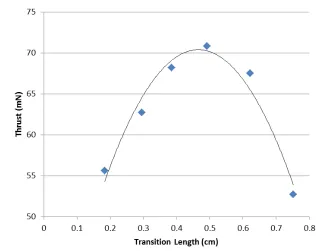
effect on performance. Figure 3-3 shows the conclusive results of these tests. There is definitely a trend on how the transition length affects performance of the jet. The optimal transition length appears to exist in the 0.45 cm to 0.55 cm range. By increasing the transition length from 0.295 cm to 0.492 cm the thrust increases 13% from 62.7 mN to 70.8 mN. A list of the data as the transition length increases can be seen in Table 3-1.
22
Table 3-1: Varying transition length data
Transition
Length(cm) Thrust (mN) Frequency (Hz) 0.183 55.6 1158
0.295 62.7 1144
0.385 68.2 1149
0.492 70.8 1149
0.621 67.5 1137
23
3.3 Inlet Optimization
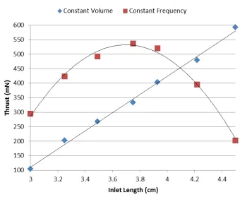
The 25 cm valveless pulsejet designed by Christian McCaulley had a unique design that allowed the inlet to be slightly modular in length. This inspired me to do a few tests based on how the inlet is designed and how to best optimize it. Figure 3-4 shows this 25 cm design. We know that the best operating pulsejet has its inlet frequency matched to its exhaust frequency [5]. I ran two sets of tests to test this theory. One involved keeping the inlet frequency the same and varying its length, while the other test involved keeping its volume the same and varying its length. Overall the inlet length was varied from 3 cm to 4.5 cm leaving the jet as 25 cm to 26.5 cm.
Figure 3-4: 25 cm variable inlet valveless pulsejet
It is important to note that the second set of tests of constant volume will yield
varying frequency. Because the jet’s operation is very closely linked to frequency matching it should be expected that the further away the inlet frequency is from the exhaust tube
24
Figure 3-5: 25 cm variable inlet valveless pulsejet thrust with trend line
25
3.4 U-Shaped Pulsejets
As described in the introduction, the valveless pulsejet has the major drawback of exhausting nearly a third of its products out of the front. The Hiller Aircraft corporation helped to solve this problem by introducing the U-shaped pulsejet which faces the exhaust and the inlet in the same direction. This is the standard shape used by hobbyists for larger valveless pulsejets today. There has not been much research in these U-shaped jets at NCSU so I have done some simulations to try and get a sense of how these jets work. The main things that were studied were the effect of the bend on the fluid dynamics, the thrust increase, and the jet’s overall ability to function. A simple U-shaped pulsejet was shown above in Figure 1-2 and was the basis for this experiment.
The main benefit of the U-shaped pulsejet is to exhaust all of the products of
combustion in the same direction. This shape also has the added benefit of allowing the user to increase the overall length of the jet while keeping a smaller form factor. For the U-shaped jets I tested the jets had an overall jet length of about 25 cm to 34 cm but the tip to bend length was still only about 12 cm. This is very helpful if the user is trying to install one of these jets into a small location. Increased length on a pulsejet generally leads to higher thrust. The benefits of having increased length are, however, offset by the increased cross sectional area, leading to a higher drag penalty. These tests were investigating the effects of having a U-shaped jet.
26
factor of about 1.8. This increase in computational time led to tests taking several weeks to run and thus these tests were more proof of feasibility.
3.4.1 U-Shaped Pulsejet Drag
27
Table 3-2: Coefficient of drag on the u-shaped jet.
Aerodynamic Propety Cd
Standard curved jet, no nose cone 0.347 Standard curved jet, with nose cone 0.285 Standard curved jet in smooth airfoil 0.249
Not surprisingly, the Cd drops with the addition of increased aerodynamics. What is interesting to note, however, is that the U-shaped jet enclosed in the smooth airfoil actually has a lower coefficient of drag than the standard straight jet. This suggests that it may be beneficial to look into enclosing a straight jet in some sort of smooth airfoil in the future.
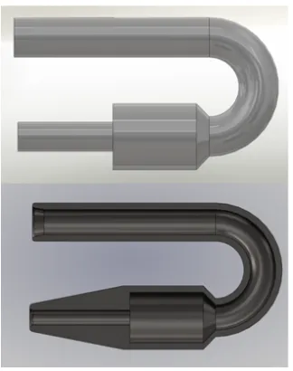
Figure 3-6: 31cm U-shaped jets. No aerodynamic cone (top) and with
28
Figure 3-7: 28cm U-shaped jet enclosed in smooth NACA 0012 Airfoil
3.4.2 U-Shaped Pulsejet Thrust
29
with the 31 cm chamber pressure is shown below in Figure 3-9. The 31 cm chamber pressure profile is much smoother and reaches the quasi-stable peak pressures as expected.
30
Figure 3-9: 25cm shaped chamber pressure (top) compared with 31 cm
U-shaped chamber pressure (bottom)
The overall thrust generated by these three curved jets is shown below in Table 3-3. In previous research we have learned to expect the valveless 25 cm pulse jet to produce thrust at approximately 400-500 mN. Because the straight jets exhaust a third of the products out of the front and two thirds out the back this leaves only a net of one third of the jets capable thrust being produced. The curved jets producing thrust on the order of 1.3 N to 1.5 N is thus very promising because it shows that the lost thrust is recovered while possibly being
31
approximately 12 cm the thrust is substantially better than the expected 90 mN of thrust on a straight 12 cm jet.
Table 3-3: U-Shaped pulsejet thrust at various lengths Jet Length (cm) Thrust (N) Frequency (Hz) Isp (s)
25 1.351 697 574.4
28 1.497 649 636.5
32
CHAPTER 4
– Valved Pulsejets
Valved Pulsejets
Valved pulsejets have the unique ability to eliminate the release of combustion products out of the front of the pulsejet. This is due to the nature of the valve mechanics themselves. A valved pulsejet places a mechanical valve directly in between the inlet and the combustion chamber. This valve opens into the combustion chamber via some sort of hinging mechanism. This means that when the combustion chamber pressure is larger than
atmospheric, as in the combustion phase, the valve will be forced shut but when it is less than atmospheric, as in the inhalation phase, it will be open. Thus, a properly designed valve will only be open when the jet is inhaling and no products of combustion will leave the
combustion chamber, greatly increasing thrust.
In general there are two types of valve dynamics mechanisms used in CFX
33
valved pulsejet performance is maximized when the valve natural frequency is slightly above the operating frequency of the pulsejet [6].
The other type of valve dynamics mechanism is the nonlinear spring which is similar to the linear valve except its valve dynamics aren’t based on the linear Hooke’s Law but rather any number of other non linear dynamics. This model is much more difficult to implement, has not been proven in simulation and is thus not presented in this project. There are some drawbacks to the valved pulsejet when compared to valveless pulsejets. They are slightly more complex than the valveless design and thus harder to implement. They are also less scalable; experimentally there have been working valveless pulsejets down to the scale of a few centimeters where as the valved pulsejet has proven incredibly difficult to get resonating at sizes less than 50 cm. Nevertheless a functioning valved pulsejet provides much improved thrust over the valveless pulsejet and is thus worth investigating.
4.1 Fuel-Air Mixture Ratio Effect
34
backwards out of the combustion chamber and through the inlet. Figure 4-1 shows this valve geometry configuration.
Figure 4-1: 12 cm 2-D valved pulsejet. Valve location highlighted in red.
In CFX you can take this fuel flow rate and specify the equivalence ratio,!, for the fuel/oxidizer ratio. This is important because it tells you how much fuel-air you are using in relation to the stoichiometric amount. The stoichiometric amount is determined by the atom balance on the chemical equation for combustion of propane, which leads to the mass of fuel to mass of oxidizer ratio to be equal to 0.275. For atmospheric conditions the mass fraction of Oxygen is about 0.232 and knowing this the mass fraction of fuel for the equivalence ratio can be solved for. The equations for equivalence ratio and propane combustion are shown below.
!= !!"#$ !!"
!!"#$ !!" !"
35
I designed a set of tests to be conducted to find the effect of running a valved pulsejet lean or rich. These tests were done on a 12 cm valved pulsejet in a 25 m/s convective stream. These tests were conducted with propane fuel at equivalence ratios of 0.7-1.1 where 1.0 is stoichiometric. The results from these tests are shown below in Table 4-1.
Table 4-1: Equivalence ratio performance results
! 0.7 0.8 0.9 1.0 1.1
Fuel Flux (g/s) 0.0167 0.0192 0.0213 0.0240 0.0258 Thrust (mN) 335.1 370.9 391.3 423.9 432.1
Isp (s) 2048.3 1966.6 1870.6 1803.3 1708.4 Frequency (Hz) 862.1 876.4 879.9 885.3 886.1
By noting the specific impulse, Isp, it is easy to see that jet performance is definitely increased by running the jet lean, but this is at the expense of losing net thrust. Not
36
4.2 Sickle Valve 3-D Simulations
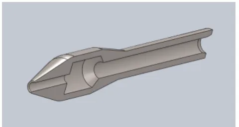
The 2-D simulations provide a good first step at simulating the valved pulsejet performance but they are quite different than the actual running pulsejet geometry. It isn’t very accurate to model the valve as simply the exact size of the valveless inlet with premixed fuel and air as the injected mass. To increase the fidelity of the simulations I’ve modeled a three dimensional valve created by Nolan Cousineau, known as the “Sickle Valve” which helps to increase mixing and swirling in the combustion chamber.
37
Figure 4-2: Sickle valve with fuel injection points (shown in red)
In the sickle valve model the fuel and air is not premixed. To achieve this I run the FORTRAN subroutine with the specification that the mass flow from the valve consist of air with a mass fraction of 0.232 Oxygen with the remaining mass as Nitrogen. The fuel is then injected as seen above in Figure 4-2, thus modeling the experimental sickle valve more closely.
38
Table 4-2: Sickle valve performance results at three fuel injection rates Fuel Flow (g/s) 0.020 0.024 0.028
Thrust (mN) 240 260 280 Isp (s) 1280 1160 1080 Frequency (Hz) 1010 1011 1016
39
CHAPTER 5
– Augmenter Effects
Augmenter Effects
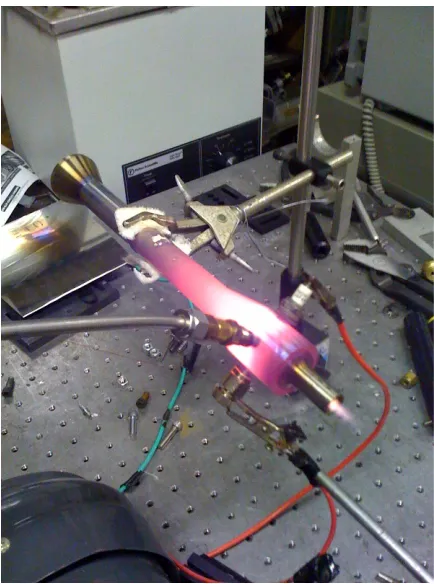
One way to increase thrust from the pulsejet is by implementing a device known as an augmenter. This device is placed behind the exhaust tube at the back of the pulsejet as seen below in Figure 5-1. The figure depicts a running, 50cm, valved pulsejet with augmenter. This setup was completely designed by Joe Scroggins. This device works by utilizing the vortex off of the end of the flare of the exhaust tube to create a low pressure zone on the inside of the lip of the augmenter. This incites entrainment of mass, pulling ambient air into the augmenter and ejecting it out of the exit. This entrainment of mass increases thrust by playing on Newton’s Second Law by increasing mass flux. The drawback of increasing the mass flux is that there is a trade off of decreased exit velocity. A well-designed augmenter, however, successfully balances this trade off by increasing mass flux more than the decrease in exit velocity [6].
40
Figure 5-1: Running 50cm, valved, pulsejet with augmenter
Figure 5-2: Augmenter location as prescribed by Fei Zheng d
L
δ
α
X
r
41
d 1.25”
D 4.34”
r 0.75”
L 10”
X 2.75”
δ 2”
α 4.64°
5.1 Effect of Forward Flight Speed on Augmenter Performance
42
the pulsejet design the bestthrust augmentation possible is only achievable in static testing because there will be no aerodynamic drag.
Experimental tests have been conducted on a 50 cm valved pulsejet and
computational simulations closely match the experimental results. I ran simulations on this 50 cm jet without the augmenter to get the baseline for the thrust produced. These tests were run with the premixed propane air valve as described in chapter 4 with a convective free stream range of 0 m/s to 40 m/s. The unaugmented valved jet produced approximately 19.5 N of thrust independent of the flow speed. I then re ran these same tests with an augmenter attached to find the thrust augmentation. A picture of this geometry is shown below in Figures 5-3 and 5-4.
43
Figure 5-4: 50 cm valved pulsejet with augmenter CAD model
5.1.1 Steady State Aerodynamic Drag
A CAD model of the optimal pulsejet with augmenter design was created for CFD tests. The first thing that was tested was how the augmenter itself responded to increasing forward flight speeds. I created a set of CFD tests on the augmenter by itself in a wind tunnel to determine how the drag increases with velocity. This is a very well understood
44
seen below in Table 5-1. From these results it is clear to see that, at low speeds, the
augmenter generates negligible drag when compared with the 19.5 N of thrust created by the unaugmented valved jet. However, at speeds above 40 m/s the augmenter generates drag on the same order of magnitude of the unaugmented thrust. At first inspection this could be where the augmenter benefits start seeing incredibly diminishing returns.
Table 5-1: Drag on augmenter alone with increasing free stream velocity Free Stream Velocity (m/s) Drag (N)
0 0.00
15 0.72
25 1.95
40 4.93
50 7.66
60 10.97
5.1.2 Augmented 50 cm Pulsejet Thrust in Varying Convective Streams
Now that the aerodynamic drag of the augmenter has been calculated it is necessary to see what augmentation is actually generated. Here the amount of “extra” thrust generated by the augmenter will be called the augmentation ration and is represented by:
45
This augmentation ratio will be used to compare how much thrust is being generated by the augmenter. Because the valved pulsejet by itself doesn’t produce any extra thrust with increased flight speed this augmentation ratio precisely gives a metric for how the augmenter increases thrust.
As seen in Table 5-2 there is significant thrust augmentation at static and low flight speeds. As the flight speed increases however, the thrust augmentation begins to drop monotonically. This should be expected due to the fact that the only reason that the thrust augmentation should drop is the increase in drag due to increased velocity.
Table 5-2: Performance of 50 cm valved pulsejet with augmenter Free Stream Velocity (m/s) Thrust of Jet Alone (N) Thrust of Augmenter (N) Total Thrust (N) Augmentation
Ratio Isp (s)
Frequency (Hz)
0 19.54 22.61 42.15 2.16 4774 245
15 18.83 11.98 30.81 1.64 3204 221
25 19.14 5.49 24.63 1.29 2632 222
40 19.54 -5.33 14.21 0.73 1661 223
The -5.33 Newtons of thrust represents that the augmenter is actually hurting the
46
Figure 5-5: Total thrust vs free stream velocity
Where the augmented jet thrust line crosses the unaugmented jet thrust line is where the augmentation ratio is equal to 1. In this case that velocity is interpolated to 32 m/s. This is the velocity where the drag of the augmenter equals the extra thrust obtained from the
augmentation. Running the pulsejet above this velocity results in a net loss in thrust. These results are somewhat unprecedented and show that for the 50 cm valved pulsejet, which is a common design amongst hobbyists, it isn’t feasible to run the pulsejet with an augmenter above 32 m/s corresponding to about 72 miles per hour.
47
determined by running the jet unaugmented and recording its thrust, then running the jet with the augmenter and determining its thrust, and dividing those two numbers. This is how the augmentation ratio was calculated above. CFX has the capability of measuring the thrust on the unaugmented jet while the augmenter is actually present. This presents a unique look at how the augmenter interacts with the jet while it is running, something not possible in the experimental case. When looking at the thrust measured at the exit of the exhaust tube on a running pulsejet with augmenter it shows that, statically, the jet has an increase in thrust. This thrust actually decreases as the forward flight speed increases and then falls below the jet alone thrust at the same point that the augmentation ratio becomes less than 1. This is surprising because the jet without an augmenter does not see any appreciable response in thrust to the increase in forward flight speed. Table 5-3 shows the thrust measured at the exit of the pulsejet but with an augmenter behind it.
Table 5-3: Thrust measured at the exit of the pulsejet with augmenter Free Stream Velocity (m/s) Thrust (N)
0 25.77
15 21.11
25 19.8
40 16.44
48
49
CHAPTER 6
– Further Experiments
Further Experiments
In addition to all of the research presented above in this paper, I have conducted a multitude of other tests to help with the design of further experimental pulsejets. These tests are useful for supplemental material and further research in the field. All of these CFD tests were designed with future work in mind.
6.1 Wind Tunnel Testing
6.1.1 Experimental Wind Tunnel
All of the experimental research done at the AERL at NCSU has been done statically, meaning there is no forward flight speed. While that is very beneficial for studying the operating nature of the pulsejet it isn’t very practical for designing something that one hopes to actually use as a means of propulsion. In the fall of 2009 we built a physical wind tunnel to help get some dynamic testing done. Figure 6-1 shows this tunnel. The wind tunnel was built with a 6” inner diameter and is capable accelerating air between 10 m/s and 30 m/s.
50
temperature of 88° F. These flow properties were used in my CFD and compared with the experimental data to test the fidelity of the computational simulations.
Figure 6-1: Wind tunnel with pulsejet on sting and dynamometer
51
extremely thin ribs allow for the transmission of any forces on the pulsejet to the dynamometer’s sensors.
Figure 6-2: Close up on dynamometer
6.1.2 CFD Wind Tunnel
52
the combination tests. Table 6-1 shows the results from these tests as well as the calculated coefficient of drag.
Figure 6-3: CFD 6” wind tunnel with 12 cm pulsejet on NACA 0012 sting
The Coefficient of drag was calculated from the following formula, the drag equation [10]:
53 Cd Coefficient of Drag D Drag Force
ρ Air Density
v Free Stream Velocity
A Pulsejet Cross Sectional Area
Table 6-1: Drag and Cd for 12 cm jet on NACA 0012 sting in 6” CFD wind tunnel
Velocity
(m/s) Drag Jet and Sting(mN) Drag Sting (mN) Drag Jet (mN) Cd
20 59.67 31.43 28.24 0.277
21 65.41 34.39 31.01 0.276
22 71.38 37.47 33.91 0.275
23 77.60 40.67 36.94 0.274
24 84.09 43.98 40.11 0.273
25 90.80 47.40 43.40 0.273
26 97.75 50.94 46.80 0.272
27 104.95 54.60 50.35 0.271
28 112.37 58.36 54.00 0.270
29 120.03 62.24 57.79 0.270
30 127.94 66.23 61.71 0.269
54
compared with the experimental data obtained from running the same jet in the wind tunnel and the plot is presented in Figure 6-4.
Figure 6-4: Drag versus free stream velocity, computational drag compared
with experimental drag
55
Nevertheless the computer model predicts, within a few percent, the drag in the overlapping areas. Because of this high correlation I did not do anymore CFD on the lower flow regimes.
6.2 Cold Flow Testing
To gain a better understanding of valve dynamics an experimental testing rig is being built to allow for viewing and recording of a valve in motion. The problem with viewing a valve in motion on a running pulsejet is that the pulsejet head normally obstructs the view of a valve often making it difficult to even see the valve in motion. Also, current pulsejets have proven to be quite difficult in reproducing consistent tests. For the purpose of studying the valve motion we want to be able to test in a controlled environment with high reproducibility.
To create this controlled environment Joe Scroggins designed a cold flow testing chamber which houses a volume the size of a normal pulsejet combustion chamber where air is pulsed through. This testing rig is designed to pull the average chamber pressure down to -7 psi while the pulsed air brings the pressure up to 14 psi. This range was decided upon as the normal operating range of a pulsejet. The chamber has threading for attaching
56
Figure 6-5: Experimental cold flow testing rig courtesy of Joe Scroggins
The cold flow testing rig is consistently going through design iterations in order to nail down the best design to produce the desired chamber pressures. Due to lack of current experimental tests on the rig I am presenting CFD of the rig to confirm feasibility of the device as well as an analysis of how it works.
6.2.1 Cold Flow CFD Testing
57
middle chamber section, and a low pressure chamber held constant at -7 psi. The inlet between the high pressure chamber and the middle chamber is a 5/8” opening. Between the middle chamber and the -7 psi low pressure chamber is a 1/2” opening.
Figure 6-6: CFD cold flow testing device
58
and only the 142 psi and 155 psi tests were able to achieve the 14 psi peak. Figure 6-7 shows the testing chamber pressure for the 123 psi, 133 psi, and 142 psi tests.
Figure 6-7: Cold flow testing at 1000 Hz for various high pressures
59
Hz the 155 psi test showed that it was able to reproduce an average test chamber of 14 psi but at individual points throughout the chamber there were spots well below 14 psi and others slightly above. This leads to the conclusion that the fluid mechanics of the device were not responding fast enough for the necessary pressure changes to occur at 2000 Hz. This isn’t a problem however because the fastest that we would want to test with this current design is for the 12 cm pulsejet head which operates in the 1000 Hz to 1500 Hz range.
These tests show that it is feasible to have this design reproduce the necessary response to drive the valve motion at 1000 Hz. From this I was able to extract the average mass flux from the high pressure side. Because these pressures and temperatures fall well within the assumptions for the Ideal Gas Law to be valid I was able to calculate the necessary high pressure chamber volume [11]. This data is shown in Table 6-2.
Table 6-2: Average mass flux and necessary high pressure chamber volume at 1000 Hz High Pressure Chamber
Pressure (psi) Average Mass Flux (g/s)
Necessary High Pressure Chamber Volume (m³)
123 13.78 1.021
133 19.09 1.420
142 25.50 1.580
155 31.80 1.741
60
61
CHAPTER 7
- Conclusions
Conclusions
The work on valveless, unaugmented and augmented valved, and curved pulsejets presents an interesting view on how these pulsejets run in varying forward flight speeds. This also leads to future work that can be done to experimentally test these jets based on the CFD presented. These are several conclusions that can be drawn from the work presented above:
• The valveless pulsejet is very inefficient when compared with a valved or curved pulsejet. They should only be used if it is the only option for running a pulsejet.
• U-shaped pulsejets indeed regain nearly all of the lost thrust due to expelling combustion products out of the inlet of the jet.
• The valved pulsejet is provides increased thrust over the valveless jet and adding an augmenter can provide additional thrust as well.
• The augmenter is useful to increase thrust only if it is below 32 m/s at which point the drag penalty is too large.
• Modeling the running pulsejet in a wind tunnel on a sting is very accurate when compared with the experimental wind tunnel data
62
REFERENCES
[1] Foa J. V. Elements of Flight Propulsion. John Wiley & Sons, New York, 1960.
[2] R. M. Lockwood. Pulse reactor lift-propulsion system development program, final report. Advanced Research Division Report No. 508, Hiller Aircraft Company, March 1963.
[3] Gunston, Bill. World Encyclopedia of Aero Engines. Cambridge, England. Patrick Stephens Limited, 1989.
[4] T. Travis, T. Scharton, A. Kuznetsov. W. Roberts. The Principles of Operation of a Pulsejet with Valves, 13th International Congress on Sound and Vibration, 2006.
[5] Thomas D. Rossing, Neville H. Fletcher. Principles of Vibration and Sound, Springer-Verlag, New York, 216-219, 2004.
[6]. Fei Zheng. Computational Investigation of High Speed Pulsejets, Doctoral Dissertation, North Carolina State University, 2009
63
[8] Robert L. Ordon. Experimental Investigations into the operational Parameters of a 50cm Class Pulsejet Engines. Master's thesis, North Carolina State University, 2006.
[9] Christian T. Mc Calley. Experimental Investigations of Liquid Fueled Pulsejet Engines. Master's thesis, North Carolina State University, 2006.
[10] Anderson, John D. Fundamentals of Aerodynamics, Fourth Edition, McGraw Hill, New York, 2007.
64
65
Appendix A: FORTRAN code for valve dynamics
#include "cfx5ext.h" dllexport(mdot1)
SUBROUTINE Mdot1 (
& NLOC, NRET, NARG, RET, ARGS, CRESLT, CZ,DZ,IZ,LZ,RZ ) CC
CD Uses value from a previous iteration in a calculation CC
CC --- CC Input CC --- CC
CC NLOC - size of current locale
CC NRET - number of components in result CC NARG - number of arguments in call CC ARGS() - (NLOC,NARG) argument values CC
66 CC
CC Stacks possibly. CC
CC --- CC Output CC --- CC
CC RET() - (NLOC,NRET) return values CC CRESLT - 'GOOD' for success
CC
CC --- CC Details CC --- CC
CC========================================================== C
C --- C Preprocessor includes C --- C
67 C ---
C Global Parameters C --- C
C
C --- C Argument list C --- C INTEGER NLOC,NARG,NRET C CHARACTER CRESLT*(*) C
REAL ARGS(NLOC,NARG), RET(NLOC,NRET) C
INTEGER IZ(*)
CHARACTER CZ(*)*(1) DOUBLE PRECISION DZ(*) LOGICAL LZ(*)
REAL RZ(*) C
68 C External routines
C --- C
C
C --- C Local Parameters C --- C
CHARACTER*20 ROUTIN
PARAMETER(ROUTIN='HEAT_SOURCE') C
C --- C Local Variables C --- C
REAL PCC, PUP, MDOT, VV, XV, DT, AIN, LIN, AV, MV, PIN INTEGER STEP
C
C initialize air conditioner to be off
69
DATA AIN/3.7476e-4/, LIN/0.0508/, G/1./, RHO/1.181/, AVX/0.0693/ DATA MV/0.00227/, AVMIN/3.7476e-6/, KV/200/, DT/1E-5/
C
C --- C Stack pointers C --- C
C=========================================================== C
C --- C Executable Statements C --- C
C
C Initialise RET() to zero.
CALL SET_A_0( RET, NLOC*NRET ) C
IF (ARGS(1,2) .NE. T) THEN DT=ARGS(1,2)-T
70 ENDIF
T=ARGS(1,2)
PCC=ARGS(1,1)
PIN=ARGS(1,3)
VV=VV+1/MV*(AIN*(PUP-PCC)-KV*XV)*DT XV=XV+VV*DT
IF (XV .LT. 0.0) THEN XV=0.0
VV=0.0 MDOT=0.0 PUP=0.0 ELSE
AV=MAX(AVMIN, AVX*XV) DO I=1,10
IF (MDOT .LT. 0) THEN
71
PUP=PCC+MDOT**2/(2*RHO)*(1/AV**2-1/AIN**2)
ENDIF
MDOT = MDOT + AIN/LIN*(PIN-PUP)*DT/10.0
IF (MDOT .GT. 0) THEN
PIN=-MDOT**2/(2*RHO*AIN**2) ELSE
PIN=0.0 MDOT=0.0 PUP=0.0 XV=0.0 VV=0.0 ENDIF
ENDDO ENDIF ENDIF
RET(1,1) = MDOT
72 CRESLT = 'GOOD'
C