ABSTRACT
UMBARKAR, TEJAS SUNIL. Computationally Efficient Simulation of Fluid-Particle Flow in Elastic Bifurcating Systems. (Under the direction of Dr. Clement Kleinstreuer).
Flows in bifurcating biomedical systems, such as the hepatic arteries and lung airways, are transient and three-dimensional. Applications of interest include the simulation and analysis of the transport and deposition of toxic or therapeutic particles in the nano- to micro-meter range. The computational resources needed for realistic, accurate and swift simulations of the particle-hemodynamics or inhaled lung-aerosol dynamics can be quite taxing. In the case of human lung-aerosol dynamics, simplified geometries, triple-bifurcation units and hybrid 3-D plus 1-D approaches have been employed (Kleinstreuer and Zhang (2009); Yin et al. (2010)).
compared with those from transient 3-D simulations (Childress et al. (2012)). The 1-D model is able to predict particle exit times with reasonable accuracy.
When assuming and incorporating more physiological, skewed velocity profiles based on bifurcating systems, the 3-D results for pressure, flow and particle exit times as well as the previous test results were even better matched.
Computationally Efficient Simulation of Fluid-Particle Flow in Elastic Bifurcating Systems
by
Tejas Sunil Umbarkar
A thesis submitted to the Graduate Faculty of North Carolina State University
in partial fulfillment of the requirements for the degree of
Master of Science
Mechanical Engineering
Raleigh, North Carolina 2013
APPROVED BY:
_______________________________ ______________________________ Dr. Clement Kleinstreuer Dr. Gregory Buckner
DEDICATION
BIOGRAPHY
ACKNOWLEDGMENTS
I convey my deepest gratitude to Dr. Clement Kleinstreuer for guiding me throughout my graduate studies. His expertise and patience helped me immensely during my work. He has always been very supportive. I would also like to thank Dr. G. Buckner and Dr. Y. Jing for serving on my committee.
Special thanks to my fellow lab-mates Miss Emily Childress, Dr. Yu Feng, Arun Varghese Kolanjiyil, Zelin Xu and Mayank Vaish for helping me out from time to time and supporting me. The discussions I had with them were very helpful in solving the problems I faced in my work.
I thank the Mechanical and Aerospace Engineering Department faculty and staff for the wonderful learning experience that I had at NC State University.
Finally I would like to thank my family and friends for standing by me. Any of this would not have been possible without the relentless support and faith put in me by my parents, both emotionally and financially.
TABLE OF CONTENTS
LIST OF TABLES ... viii
LIST OF FIGURES ... ix
CHAPTER 1 INTRODUCTION ...1
1.1 Research Objectives ...1
1.2 System Description ...3
1.3 Literature Review ...5
1.3.1 Computational Analysis ...5
1.3.2 Experimental Evidence ...7
1.3.3 Modeling Approaches ...8
1.4 Summary and Conclusions ...14
CHAPTER 2 MODEL DESCRIPTION OF FLUID FLOW ...16
2.1 Introduction ...16
2.2 Theory ...16
2.2.1 System of Equations and Fluid Structure Interaction (FSI) ...17
2.2.2 Boundary Conditions ...20
2.2.2.1 Windkessel Models ...22
2.2.3 Numerical Scheme ...25
2.3 Trial Run ...29
CHAPTER 3 PARTICLE DYNAMICS ...37
CHAPTER 4 VALIDATIONS AND RESULTS ...42
4.1 Introduction ...42
4.2 Validation with the Aortic Model of Alastruey (2006) ...42
4.2.1 The Model ...42
4.2.2 Boundary Conditions ...44
4.2.3 Implementation ...46
4.2.4 Simulation with Bifurcation Conditions ...50
4.3 Validation with Experimental/Computational Observations by Kung et al. (2011) ...54
4.3.1 The Experiment ...54
4.3.2 The Simulation ...55
4.3.3 Parameters Used in Our Model ...56
4.4 Validation with the Model by Marchandise et al. (2009) ...60
4.4.1 Model Details ...60
4.4.2 Boundary Conditions ...61
4.4.3 Implementation ...62
4.4.4 Results ...62
4.5 Conclusions ...64
4.6 Results ...65
4.6.1 Model Details ...65
4.6.2 Boundary Conditions ...67
4.6.3 Implementation ...68
4.6.5 Particle Transport ...78
4.6.6 Particle Exit Fractions ...80
4.7 Skewed Velocity Profile ...81
4.7.1 Derivation of the Skewed profile ...81
4.7.2 Applications ...86
4.7.3 Previous Validations ...89
4.8 Concluding Remarks ...92
CHAPTER 5 CONCLUSIONS AND FUTURE WORK ...93
5.1 Conclusions ...93
5.2 Limitations and Future Work ...95
REFERENCES ...97
APPENDICES ...102
APPENDIX A ...103
LIST OF TABLES
Table 2.1 Geometrical parameters for the single bifurcation ...29
Table 4.1 Length and radii of the nine arteries ...66
Table 4.2 WK2 parameters used in 3-D comparison ...68
Table 4.3 Comparison of 1-D and 3-D particle exit times for the outlets ...79
Table 4.4 Particle exit fractions for 1-D and 3-D ...80
LIST OF FIGURES
Fig. 1.1 Visual representation of the coupled 3-D/1-D model ...2
Fig. 1.2 Major arteries in the human circulatory system ...4
Fig. 1.3 A representative model of the CHA and its daughters ...4
Fig. 2.1 The axial velocity profile assumed by Olufsen et al. (2000) ...17
Fig. 2.2 Historical Windkessel application ...22
Fig. 2.3 Physiological representation of a two element Windkessel Model ...23
Fig. 2.4 Electrical representation of two and three element Windkessel models ...24
Fig. 2.5 Geometry of the single bifurcation ...30
Fig. 2.6a,b Initial conditions for bifurcation ...31
Fig. 2.7 Area at various time steps for the vessels...32
Fig. 2.8 (a)- Pressure in CHA (b)- Flow in CHA after 1500 time steps ...33
Fig. 2.9 Flows in the three vessels at 2250 time steps ...33
Fig. 2.10 Pressures in the vessels at 2250 time steps ...34
Fig. 2.11 (a)-Pressure in GDA and PHA, (b)-Flow in GDA and PHA at 3000 time steps ...35
Fig. 4.1 Visualization of the aortic model ...45
Fig. 4.2 Comparison of numerical results for pressure with those of Alastruey ...46
Fig. 4.3 Comparison of numerical results for flow with those of Alastruey ...47
Fig. 4.6 Pressure for run with bifurcation conditions ...50
Fig. 4.7 Flow plot for run with bifurcation ...51
Fig. 4.8 Pressure for run with E=5.2 x10⁵ Pa ...52
Fig. 4.9 Flow plot for run with bifurcation conditions with E=5.2 x10⁵ Pa ...52
Fig. 4.10 The experimental set up as given in Kung et al. (2011) ...54
Fig. 4.11 Physiological flow input to the model (Kung et al. (2011)) ...55
Fig. 4.12 Pressure plot for E= 1 MPa, r0= 1 cm. ...56
Fig. 4.13 Flow plot for E= 1 MPa, r0= 1 cm. ...57
Fig. 4.14 Pressure plot for E= 1.2 MPa, r0= 1 cm. ...58
Fig. 4.15 Flow plot for E= 1.2 Mpa, r0= 1 cm ...58
Fig. 4.16 Change in radius for E= 1.2 MPa, r0= 1 cm ...59
Fig. 4.17 Geometry for validation of the bifurcation ...61
Fig. 4.18 Pressure plots from 1-D and those of Marchandise et al. (2009) ...63
Fig. 4.19 Representative 3-D Hepatic Arterial System ...65
Fig. 4.20 Inlet flow waveform for 3-D and corresponding 1-D simulation ...67
Fig. 4.21 Comparison of 3-D and 1-D pressure and flow for the nine vessels ...70
Fig. 4.22 Comparison of 3-D and 1-D pressure and flow for the nine vessels with representative elasticity ...75
Fig. 4.23 Geometry used for extracting the velocity profile ...82
Fig. 4.24 Sites for evaluating the velocity profiles with their angular location ...82
Fig. 4.25 Average normalized velocity profiles at different angular positions. ...84
Fig. 4.27 Comparison between boundary layer profile
and skewed profile for pressure and flow ...88 Fig. 4.28 Comparison between skewed profile and results from Kung et al. (2011) ...90 Fig. 4.29 Comparison between skewed profile and results from Alastruey (2006) ...90 Fig. 4.30 Comparison between skew profile
CHAPTER 1
INTRODUCTION
1.1 Research Objectives
A novel technique has been proposed by Kleinstreuer et al. (2012) and further analyzed by Childress et al. (2012) for targeting drugs onto liver tumors. In this third-level treatment option, radioactive microspheres (typically of yttrium 90) are released from a smart catheter which can be optimally placed in the common hepatic artery or the proper hepatic artery. These microspheres then travel through the hepatic vasculature and either embolize the smaller arteries connecting to the tumor, cutting off blood supply, or with their radioactivity they can kill the tumor cells upon deposition. However, this radioactivity can also kill healthy tissue or the microspheres can block vessels leading to other healthy organs, causing unwanted damage to the body. Thus, it is required that these microspheres be ‘targeted’ to a particular upstream artery which is connected to the tumor.
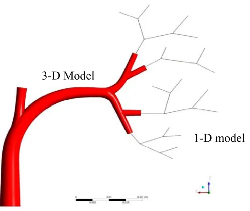
to develop a 3-D/1-D coupled model. In this, the first few generations of the arterial system would be modeled in full 3-D. For the further downstream generations, a 1-D model would be used (see Fig. (1.1)).
Fig. 1.1 Visual representation of the coupled 3-D/1-D model
This would not only reduce computational efforts, but also increase the range of our simulations beyond that of the available 3-D geometry.
Thus, the objectives of this study are as follows:
1. Development of a 1-D model to simulate the flow, pressure, wall movement and particle trajectories in elastic arterial systems.
2. This model should be able to obtain reasonably accurate results with minimal 1-D model
1.2 System Description
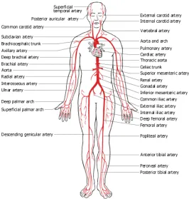
The human body contains millions of arteries. These arteries (except the pulmonary and the umbilical artery) carry oxygenated blood from the heart to the different organs in the body. When any of the branches of the artery bifurcate, it is called a generation of the vessel. At every generation the radii of the daughter vessels are smaller than that of the parent vessel; however, the total area of the daughter vessels is greater than the area of the parent vessel of the previous generation. The number of generations and the anatomy of the arterial system is highly patient-specific. The artery walls are composed of three layers, i.e., the Tunica Extrema, Tunica Media and Tunica Intima. These make the arteries flexible and even viscoelastic in nature. Due to this, the arteries change their diameter as the pressure in them changes throughout the pulse. This is the reason we can ‘feel’ the pulse. The vessels taper in their diameter. Also, their elasticity is not constant. It can change with the radius of the arteries as well as the pressure inside them. Figure (1.2) shows the general structure of the arterial tree.
Fig. 1.2: Major arteries in the human circulatory system (from American Medical Association website)
GDA
RHA
LHA CHA
A computer model of this arterial system is a very useful tool in disease investigations and remedial solutions. However it is difficult to model the entire system with all its complexities in 3-D all the way up to the sinusoids. Hence the general idea is to have a 3-D model for the first couple of generations and then extend via 1-D modeling of the vessels. The pressure and flow characteristics can be simulated satisfactorily, using this 3-D/1-D approach. Generally, appropriate boundary conditions are used in place of downstream vessels, after 1-D modeling of a few generations of vessels.
1.3 Literature Review
1.3.1 Computational Analysis
Another 3-D/1-D coupled model has been presented by Formaggia et al. (2001) for fluid flow in a compliant vessel. They discussed strategies for coupling the 3-D and 1-D equations and presented numerical results for a simple case of a flexible straight tube.
Olufsen (1998) proposed a 1-D model involving a reduced and modified form of the Navier-Stokes (N-S) equations. The author discussed in detail the ‘structured tree’ outlet boundary condition. The human systemic arterial structure was divided into two parts: the large arteries and the small arteries. The large arteries were modeled as a binary tree from the geometric data obtained from MRI scans while the small arteries were modeled as structured trees. The blood flow and pressure were calculated only in the large arteries. The smaller arteries (structured tree) were modeled in the frequency domain and analytical solutions of the N-S equations were obtained. The impedance of the structured tree to the flow was obtained from this which was then used as an outlet boundary condition for the larger arteries.
Reymond et al. (2009) proposed a model incorporating a heart model, detailed cerebral and coronary arterial systems, non linear and viscoelastic behavior of vessel walls and realistic outflow boundary conditions. The results were then compared with experimental flow and pressure waveforms from healthy individuals. They also gave a brief on the different models present for 1-D simulation and their components.
Formaggia et al. (2003) conducted a mathematical analysis of the 1-D system. They analyzed a domain decomposition method for handling branching and prosthesis attachments to the arteries. They also discussed the effect of branching angle of the daughter vessels.
Similar 1-D models have been developed by van De Vosse and Stergiopulos (2011) and Sherwin et al. (2003) among others. All the above models differ in the variables of the basic equations and the way in which the physical aspects are implemented, which would be discussed later. A general observation from these publications is that the 1-D model is able to predict the flows physiologically.
1.3.2 Experimental Evidence
While the above mentioned articles focus mainly on computational work, experiments have also been carried out to obtain pressure and flow waveforms in the arterial system, useful for validation of computer models.
the assembly easily. The diameter and thickness of the phantoms were selected to match those of the descending thoracic aorta. They attached a four element Windkessel model as the outlet BC. The resistance module was constructed by placing in parallel a number of capillary tubes while a plexiglass chamber trapping a precise amount of air was used as the capacitance. A physiological inlet flow waveform was applied with the help of a computer controlled pulsatile pump, the working fluid being a 40% glycerol solution.
A model of the systemic arterial tree consisting of the 37 largest arteries was constructed by Matthys et al. (2007). These vessels are tapered and are made of a two component silicone material. A Harvard pump was used to apply the pulsatile input while the outlets are connected to resistance tubes. The working fluid was again a 35% glycerol solution.
Segers et al. (1998) constructed a larger tree consisting of 55 of the largest arteries. The material used for the vessels was latex rubber. The outlet resistance was modeled by porous rubber in syringe and the compliance was modeled by a syringe with an air chamber. This peripheral module was connected to a tube which connected to an overflow system giving a constant venous pressure. This model has been used by Alastruey (2006) and Olufsen (1998) in their studies.
1.3.3 Modeling Approaches
contracting in cross sectional area with changes in pressure and also the impact of elastic or viscoelastic vessel walls. The main differences between different modeling approaches are the way in which they implement the boundary conditions, the relation between pressure and area and the discretization scheme.
The most basic component of the model is the set of 1-D N-S equations. Olufsen et al. (2000) derived these equations in integral form of the conservation equations. Circular arteries were assumed. They derived the mass and momentum conservation equations with the vessel area and flow as the variables. A flat ‘plug flow’ profile was assumed. Sherwin et al. (2003) derived these equations in several different combinations of variables as given below:
A-Q form:
0
/
A-u form:
0
/2 1
p-u form:
1
0
/2 1
p-Q form:
1
0
/
Here, f represents the frictional force per unit length. However, there are certain assumptions involved in deriving the other forms of equations. The A-u and p-u forms assume inviscid flow while the p-Q form assumes constant material properties. The A-Q form is thus the most general form among these. Formaggia et al. (2003) also develop a similar set of equations in the A-Q form.
Along with the governing equations, an important component is the fluid-structure interaction (FSI) model. As mentioned earlier, the arteries are flexible and their cross-sectional area varies with the pressure inside them. In a single pulse the pressure varies from diastole (~80 mmHg) to systole (~120 mmHg), which means that the area of the arteries would be changing. To include this phenomenon, a FSI model is needed. Formaggia et al. (2003) provide a comprehensive relation between the pressure and the area of the vessel in terms of a partial differential equation representing the mechanical model for wall displacement.
1.1
with this relation complete the system of equations for p, A and Q. A simplified p-A relation is also used by other authors like Sherwin et al. (2003), Olufsen (1998) and Alastruey (2006). Reymond et al. (2009) also present a viscoelastic model for vessel walls. They assumed that the vessel area at any location is the sum of a nonlinear elastic component and a viscoelastic component.
For accounting the change in elasticity with radius, Olufsen et al. (2000) used an exponential relation between the elasticity and radius. However, other authors mentioned above do not use any model for the elasticity but use the elasticity of each vessel from measured values. It should be noted that we might not always have the values or data for knowing the elasticity of certain further downstream vessels.
Alastruey (2006) and Sherwin et al. (2003) employed a discontinuous Galerkin numerical scheme with a high-order 1-D spectral/hp element spatial discretization. They then used the second order Adams-Bashforth time integration scheme. Formaggia et al. (2003) used a second order Taylor-Galerkin scheme. Olufsen (1998) and Smith et al. (2002) applied a two-step Wendroff scheme while Formaggia et al. (2001) used a standard Lax-Wendroff scheme. Ho et al. (2009) used the finite difference MacCormack scheme.
bifurcations of the vessels. Reflection coefficients have been used by Reymond et al. (2009) and Wang and Parker (2004).
As mentioned earlier, the 1-D equations will not be used all the way up to the sinusoids. The model has to be terminated at a certain point and appropriate outflow BC should be used in order to replace the vasculature downstream. This BC should be able to capture the wave propagation and reflection phenomenon caused due to the downstream vasculature. A general approach is to represent the flow resistance, inertia and vessel distensibility with electrical counterparts i.e. resistance, inductance and capacitance. Debbaut et al. (2011) replaced the Navier Stokes equations with four components of a pi-filter for each of the vessel segments. These four components (Rs, L, C, Rp) represent the longitudinal resistance, blood inertia, vessel compliance and vessel viscoelasticity respectively. The four elements of the pi-filter were functions of the physical properties like blood density, viscosity, vessel compliance, radius, length etc. This approach is similar to the Windkessel model which is another type of outlet BC and will be explained in later sections. This is used by Alastruey (2006) and Kung et al. (2011) among others. Grinberg and Karniadakis (2008) discussed the resistance, impedance and Windkessel BC. They suggested a time dependent resistance (R(t)C) method which they successfully compared with the impedance BC. This method was similar to the two-element Windkessel except for the fact that the resistance used here is time dependent.
each terminal vessel and branched off with specific daughter branch diameter ratios. The lengths were also determined from radius/length ratios. The fluid dynamic equations for the vessels of the structured tree were written in a frequency domain using Fourier transforms. An analytical solution of the system was found and from that the root impedance of the tree is found. The impedance is calculated by:
, ,
, 1.2
0,0 8 , 0 1.3
where p(x, ω) is the pressure, Q(x, ω) is the flow and Z(x, ω) is the impedance at frequency
ω.
From Equation (1.2), we see that Z is proportional to 1/r3. Each structured tree is grown until a certain minimum radius rmin is reached. This minimum radius is adjusted so as to give an appropriate value for the impedance which gives near physiological values at the inlets. Since different body parts will have different peripheral resistance, each structured tree would have a different rmin or we can keep the same rmin and apply different terminal impedance to the structured tree and propagate it upstream in the structured tree. At bifurcations, the impedances of the vessels are in parallel hence the impedance of the parent vessel is found out by:
1 1 1
1.4
After finding Z(0,ω), i.e. the impedance at the outlet of the main vascular tree arising due to the structured tree (the root impedance), the impedance in the time domain (Z(0,t)) can be found out by inverse Fourier transform. This method is however, computationally expensive.
1.4 Summary and Conclusions
1. A 1-D system is fully capable of reproducing the flow and pressure waveforms in a flexible arterial system.
2. Different paths can be followed depending upon the selection of the method of generating the geometry, form of the governing equations, p-A relationship, types of outflow BCs, and the discretization scheme.
3. The governing equations can be written in (A, u), (A, Q), (p, u) and (p, Q) forms. Out of these the (A, Q) form developed by Olufsen (1998) is the most general form with fewer assumptions.
5. The arterial system cannot be modeled all the way up to the capillaries. At some point, the arterial tree has to be truncated and suitable outlet BCs have to be implemented to satisfy the physiological conditions.
CHAPTER 2
MODEL DESCRIPTION OF FLUID FLOW
2.1 Introduction
Based on the conclusions of the literature review given in the previous chapter, most suitable modeling equations and associated boundary conditions are selected for a representative arterial tree. Specifically, a description of the model and its coding are provided, and the use of appropriate parametric outflow boundary conditions for a structured tree, as originally proposed by Olufsen et al. (2000), are discussed.
2.2 Theory
The process of building the 1-D model consists of several steps of choosing the right parameters and procedures. The principal topics of interest are:
1. The system of equations.
2. The relation between the vessel area and pressure, i.e. fluid-structure interaction (FSI). 3. The boundary conditions.
4. The numerical scheme.
2.2.1 System of Equations and Fluid Structure Interaction (FSI)
As outlined in Chapter 1, Olufsen et al. (2000) started with the Navier-Stokes equations and then simplified those, using averaged quantities. For example, human arteries taper along their length. To account for this fact, radial vessel variations are assumed as follows.
2.1
where r(x) is the (base) radius at any point along the length x of the vessel, rin is the inlet radius, rout is the outlet radius, and L is the length of the vessel.
To obtain the 1-D form of the governing equations, certain assumptions have to be made. It is assumed that the pressure is constant over the cross-section and then the velocity is integrated over the cross-section. Hence, a ‘plug flow’ velocity profile results.
,
, 2.2
Here, u(r) is the radius dependent axial velocity in the vessel, and u is the cross-sectionally averaged velocity.
Fig.2.1 The axial velocity profile assumed by Olufsen et al. (2000)
δ
u r
The final form of the 1-D N-S equations are (see Appendix):
0 2.3
2
2.4
where Q= volume flow rate, A= area, = kinematic viscosity, = boundary layer thickness (for larger vessels = 0.1 cm), R= radius of the vessel, and R=R(x, t). It is assumed that the density and viscosity are constant, pressure p is constant along the cross sectional area and the vessel is longitudinally tethered i.e. the vessel can only vary in radial direction due to compliance. It is assumed that there is no velocity-slip at the walls. Equation (2.3) is the continuity equation, while Equation (2.4) is the momentum equation. Similar expressions as those of (2.3) and (2.4) were also obtained by Sherwin et al. (2003) and Alastruey et al. (2008). The N-S equations can also be written in terms of area and velocity, or pressure and velocity, or pressure and flow rate (Sherwin et al. (2003)). However, the expressions in terms of area and flow rate are easier to work with and require the fewest assumptions.
We observe that in the above system, there are two equations but three variables (A, Q, p). So, we need a third equation to complete the system. This third equation is called the state equation and it provides the relation between the area and pressure in the vessel (FSI). As explained in Section 1.3.3 Formaggia et al. (2003) proposed a comprehensive mechanical relation for the FSI considering the viscoelasticity of the arteries:
The N-S equations along with this relation complete the system of equations for p, A and Q. However, implementing the mechanical relation in its complete form is very difficult. Hence, the authors first neglected all the partial derivatives in the mechanical relation (2.6) and obtained a purely algebraic relation between p and A. This relation is:
√
, √ , √
√ 2.6 , ,
In the above relations, h0 and A0 is the reference thickness and area of the vessel, respectively; E is the Young’s modulus and pext is the external pressure; and η is the displacement of the vessel wall with respect to the reference configuration. They then compared their results by including the different terms in the mechanical relation (2.5) and finally concluded that for physiological values of pressure and velocity, these terms can indeed be neglected and a simple algebraic expression can be used between p and A. Olufsen (1998) uses a similar relation as:
, 4
3 1 √ 2.7
where , and are the pressure, radius and area at zero transmural pressure, i.e., diastole, respectively. Olufsen (1998) assumed the arteries to be tapering thin-walled vessels and then the internal and external forces are balanced in the radial direction to get the above relation between the pressure and the cross-sectional area.
The elasticity of the vessels is required for estimating their compliance, i.e., their tendency to expand and contract according to pressure changes. The compliance is given by:
3
Stergiopulos et al. (1992) have published data for the volume compliance of various human arteries. From this data Olufsen (1998) derived an expression for the combined parameter Eh/r0 as:
2 10 exp 2253 8.65 10 2.9
Knowing completely the p-A relationship, we can now substitute it into the system (2.3)-(2.4) and move ahead to its numerical solution.
2.2.2 Boundary Conditions
Three types of boundary conditions are required for the inlet, bifurcations and outlets to close this hyperbolic system, i.e., Equations (2.3) and Equation (2.4). We must first find the values of the variables at all the boundaries to be able to calculate the flow field in the interior.
The inlet boundary condition is fairly straightforward as the inlet values for either mean velocity or flow rate would be known. The value of the other variable (i.e., area) at the inlet can be calculated from this data.
The outlet boundary condition is trickier than the other ones. We need to find a suitable model which would simulate the appropriate impedance characteristics and wave reflections of the downstream vessels, which are being replaced by the BC.
Olufsen et al. (2000) employed the structured tree outlet BC (see Section 1.3.3). The authors claimed that this BC is a physiologically correct BC and is better than the generally used Windkessel BC as it is able to capture the reflected waves effectively and able to maintain a ‘phase lag’ between the pressure and flow. The structured tree can also capture the high frequency oscillations (Olufsen (1999)). However, the Windkessel is much easier to use and gives physiological results very similar to those obtained from the structured tree BC.
Another similar approach has been followed by Lin et al. (2009) for the geometrical modeling of the pulmonary airways. They placed a grid of uniformly spaced seed points within each lobe of the lung, the geometry of which was obtained from imaging techniques (Tawhai et al. (2004)). Then, the image-based peripheral airways were used as starting points and branching was done in the following manner:
1. The closest end point on a peripheral branch is calculated for each of the seed points. 2. Thus, there will be as many sets of seed points as there are peripheral branch end points. 3. Each set is divided into two by a line passing through the center of mass and the end
point and the center of mass of each of the two parts is calculated.
4. A branch is generated by starting at the end point directed towards the center of mass of that part, with length equal to 40% of the length between the end point and the center of mass.
The diameters of these branches were then decided from the equation:
log log log 2.9
where D(x) is the computed diameter for any branch of Strahler-order x, N is the highest order (order of trachea), DN is the diameter of the branch with highest order, and RdS is the diameter ratio (antilog of the slope of plot of log(mean diameter) against Strahler-order).
The N-S equations can then be solved for these generated vessels to obtain the required outflow BC at the end of the larger vessels.
A third possible BC is the Windkessel boundary condition which is adopted in this work. The details are given in the next section.
2.2.2.1 Windkessel Models
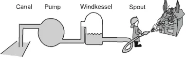
The Windkessel model was first proposed by Otto Frank in 1899 in order to simulate the flow and pressure waveforms in arteries. The idea originated from the concept of air-vessels used in fire trucks.
The air-vessel stores energy during the pumping stroke of the reciprocating pump and releases it during the non-pumping stroke, thus pumping water through the spout even during the non-pumping stroke. The same idea is applied for the vascular system. The vessels, being elastic, expand during the systole, storing blood volume and then release this volume during the diastole. This effect is captured by the Windkessel model (WK). This is a lumped capacitance or 0-D model, meaning that it assumes constant (average) variables for the entire vessel or group of vessels. It does not have spatial resolution for a particular vessel. Its physiological representation is as follows:
Fig. 2.3 Physiological representation of a two element Windkessel Model (adopted from Westerhof et al. 2009).
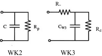
The WK can also be represented by an equivalent electrical circuit. The initial model consisted of only two elements: a resistance representing the total resistance to the flow and a capacitance representing the compliance of the vessels.
Heart Compliant
vessels (WK)
Fig. 2.4 Electrical representation of two and three element Windkessel models. Rp- total peripheral resistance, C- total systemic arterial compliance, CW3- total arterial compliance for the three-element WK, Ru- characteristic impedance, and Rd=Rp-Ru (adopted from Burattini,
Natalucci (1998)).
Thus, the flow corresponds to the electric current and the pressure difference corresponds to the voltage drop. This simple model was able to predict the pressure decay in diastole but failed in systole. An improvement over the two-element WK (WK2), a three-element WK (WK3) was proposed which included an additional characteristic resistance (Westerhof et al. (2009)). Further refinement can be done by adding a fourth element that is the inductance representing the blood inertia either in series (WK4s) or in parallel (WK4p) to the characteristic resistance (Segers et al. (2008)). Not surprising, a study by Stergiopulos et al. (1999) showed that WK4 is more accurate than WK3. Another study by Segers et al. (2008) showed that when comparing WK3 and the two WK4 models, the WK4s provided the best fit for the available flow data. However, it is computationally demanding and the inductance is difficult to estimate. After analyzing their results for WK3, it was found that there is not much difference in the accuracy of WK3 and WK4s models. Also, Westerhof et al. (2009)
WK2 WK3
Ru
entrance of the arterial system. Alastruey et al. (2008) investigate R, RCR, CR and LR models for outlet BC and finally conclude that the RCR i.e. three element Windkessel model can efficiently represent the physiological BC. Hence, owing to the ease of formulation and equivalent accuracy, the WK3 was used as the outlet BC.
The electrical circuit of WK3 can be solved with help of Kirchhoff’s laws and Ohm’s law and the final relation between the parameters of the circuit is obtained as:
1
1 2.10
where Q is the flow rate through the system being replaced by the WK3 and p is the pressure.
2.2.3 Numerical Scheme
Among the different schemes discussed in Section 1.3.3, the two step Lax-Wendroff scheme was selected for its simplicity (Olufsen et al. (2000)). It is a second-order method in both space and time. The general formula for this method is as follows.
For the hyperbolic system,
, , 2.11
The first step,
2 1
2 ∆ ∆
2.12
∆ ∆ 2.13
Finally, our specific hyperbolic system (Equation (2.3) and Equation (2.4)), after incorporating the pressure-area relationship (Equation (2.7)) is:
0 2 √
√ 2√ √
1 2.14 ,
where, Q=flow rate Q(x,t), A=area A(x,t), A0=area at zero transmural pressure A0(x), function f=(4/3)Eh/r0, r0(x)= inlet radius x (outlet radius/inlet radius)x-distance/length of vessel , = boundary layer thickness (assumed to be 0.1 mm from Olufsen et al (2000)). This system is in the form:
2.15
where the vectors U, R and S can be obtained by comparison with Equations (2.14a, b). This results in a numerical Lax-Wendroff scheme of the form:
∆ ∆
∆
2 2.16
The values of the variables at the intermediate time steps can be found by:
/ /
2
∆
The code has been written in FORTRAN 95 (Microsoft Visual Studio 2005). The choice of the coding language was made based on the ease of incorporation into commercial packages like ANSYS CFX for further processing. All the vessels are divided into equal number of parts and flow and pressure are calculated for each of these parts. In general, the subscript specifies the position in space and the superscript specifies the time step. At the inlet, the flow rate is known at all time steps i.e. is known at any n. Observing Equation (2.16) and Equation (2.17), we see that in order to find the inlet area, i.e. , we need to introduce a ghost point at n= -1/2. It is found out as follows:
1
2 2.18
Here, is known from the inlet BC and can be found out from Equation (2.15). As
mentioned earlier, across a bifurcation the pressure is constant and the flow is conserved, i.e.
, , , 2.19
And
, , , 2.20
The flow is conserved across a bifurcation:
, , , 2.21
And
, / , / , / 2.22
/ / /
2 2.23
and
/ / /
2 2.24
Where i=L for parent vessel and i=0 for the daughter vessels.
An equation similar to Equation (2.16) can be written for the end point of the parent and the inlet point for the two daughters, for area and flow each. This gives us six equations. Equations (2.19) through (2.24) along with the six forms of Equation (2.16) mentioned above constitute a non-linear set of 18 equations involving 18 variables listed below:
1 , 2 , 3
,
4 , 5 , / 6
, /
7 , 8 , / 9
, /
10 , 11 , 12
,
13 , 14 , / 15 , /
16 , 17 , / 18
, /
With being the variable vector (18 x 1) at the (k+1)th iteration, is the inverse of the Jacobian matrix (18 x 18) for the corresponding residual equation matrix .
For the outlet, a procedure similar to that for inlet is used. In this case, a ghost point is assumed after the last grid point of the vessel, i.e. at L+1/2 and calculations are done. The outlet pressure or flow is known form the WK3 BC. It is discretized as (see Equation (2.10)):
∆
∆
1
1 2.26
From this pressure, we are able to calculate the area at the outlet (from the pressure-area relationship) and the flow at the outlet (through the fluid dynamical expressions) for the next time step.
After the application of the BC, we now have all the boundary values at the (n+1)th time step and can now proceed with the application of the numerical scheme on the interior points using equations (2.16) and (2.17).
2.3 Trial Run
Table 2.1 Geometrical parameters for the single bifurcation. *Value taken from Olufsen et al. (2000), **Arbitrary value. All other values from Basciano (2010)
Length (m) Inlet radius (m) Outlet radius (m)
CHA 0.028 0.003 0.0025*
GDA 0.028** 0.0015 0.0013**
PHA 0.027 0.0022 0.0020**
Fig. 2.5 Geometry of the single bifurcation
A Gaussian flow waveform was prescribed at the inlet.
exp 200 n 1 0.2 10 2.27
be 1060 kg/m3 and viscosity was assumed to be 0.003090 kg/m/s. The code was run with a Courant-Friedrichs-Lax (CFL) number of 0.075 and 100 grid points for each vessel. An absorbing BC was used as the outlet BC.
The code uses a global time step for all the grid points which is updated at each time step. The following plot shows the initial condition for the problem, which was assumed to be the same for all vessels.
(a) (b)
Fig. 2.6a,b Initial conditions for bifurcation. (a)-area, (b)-flow
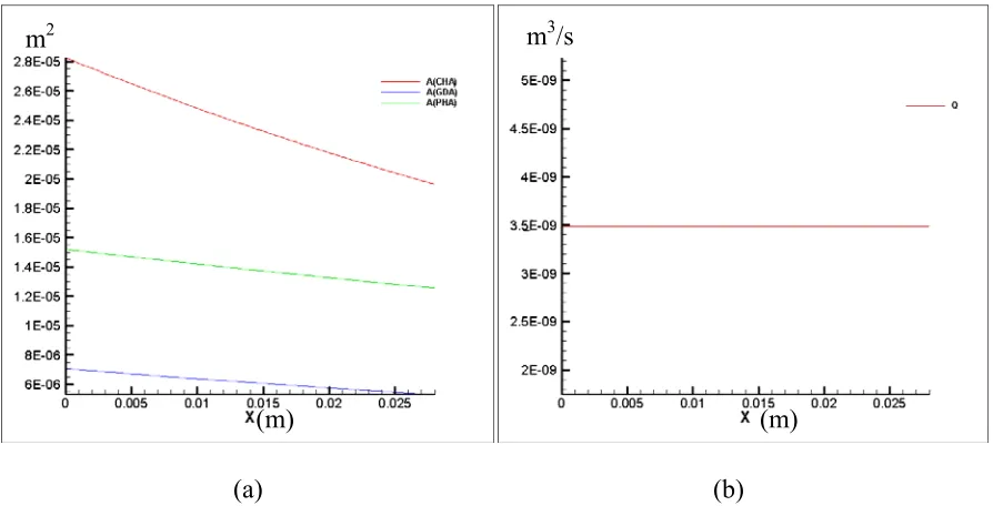
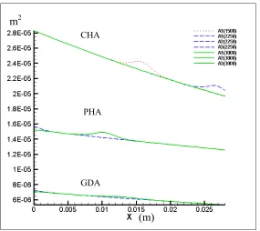
The code was then run for 3000 time steps and the corresponding flow rates, areas and pressures were plotted. The following graphs of Fig. (2.7) depict how the input pulse propagates though the bifurcation, with the following abbreviations:
A1-area of CHA Q1- Flow in CHA P1-Pressure in CHA
m2 m3/s
A2-Area of GDA Q2-Flow in GDA P2-Pressure in GDA
A3-Area of PHA Q3-Flow in PHA P3-Pressure in PHA
Values in brackets indicate number of time steps.
Fig. 2.7 Area at various time steps for the vessels
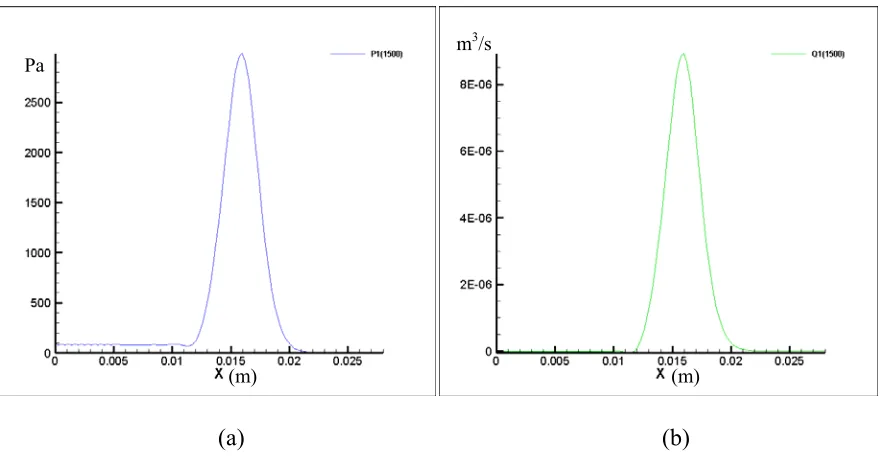
This figure shows the change in area as the pulse moves through the vessels. At 1500 time steps, the pulse is just about halfway through the CHA. Hence there is no effect on the PHA and GDA. But after around 2250 time steps, the pulse moves through the bifurcation and its effect can be seen in the daughter vessels. Figure (2.8) provides the pressure and flow in the CHA after 1500 time steps.
m2
(m)
CHA
PHA
(a) (b)
Fig. 2.8 (a)- Pressure in CHA, (b)- Flow in CHA after 1500 time steps.
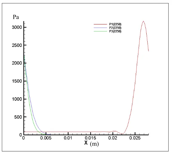
Fig. 2.9 Flows in the three vessels at 2250 time steps.
Pa m
3/s
(m) (m)
m3/s
This plot shows the transition of the flow through the bifurcation from the CHA into the GDA and the PHA. It can be estimated from the plot that the sum of flows at the inlet of the two daughters is equal to that at the outlet of the parent. The flow in the GDA is smaller than that in the PHA, as the flow area of the GDA is smaller than that of the PHA.
Fig. 2.10 Pressures in the vessels at 2250 time steps.
The above plot represents the pressures in the vessels as the wave travels through the bifurcation. It can again be verified that the pressures at the inlet of the two daughters is equal to that at the outlet of the parent.
(a) (b)
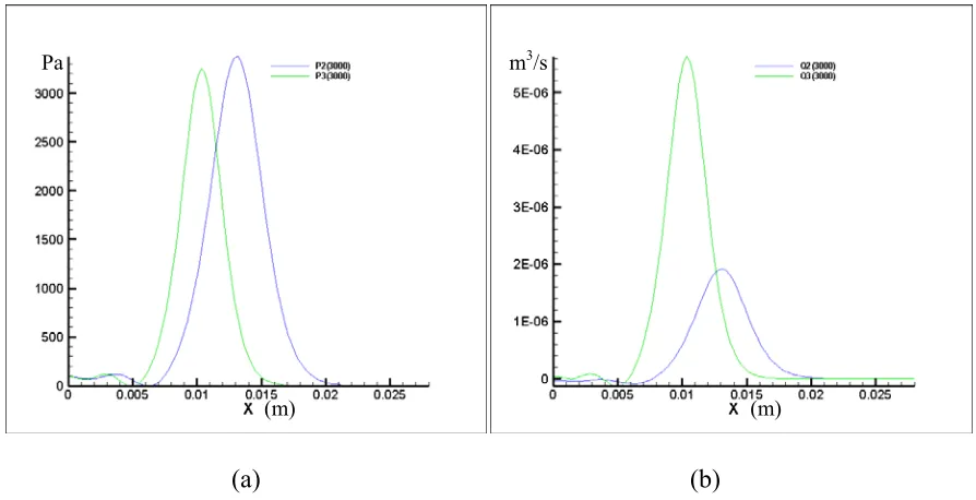
Fig. 2.11 (a)- Pressure in GDA and PHA, (b)- Flow in GDA and PHA at 3000 time steps
The plots in Fig. (2.11) represent the pressure and flow profiles in the PHA and the GDA after 3000 time steps. At this stage, the wave has completely passed the bifurcation. It can be seen again that the magnitude of flow in the GDA is smaller than that in the PHA due to the corresponding flow areas. However a reverse trend is found in the pressure plots. This is again due to the fact that the flow area being lower in the GDA, the peak pressure is higher. We can also observe that the pressure and flow profiles in the GDA are further advanced in space as compared to those of the PHA. This can be attributed to the fact that the pressure being higher in the GDA, the flow velocity is also higher and hence, the flow advances further than that in PHA for the same time. Also, the GDA has a smaller radius than PHA which means that in our elasticity model, GDA will have a higher elastic modulus than PHA, which would increase the wave speed in GDA (Olufsen (1998)).
Pa
(m)
m3/s
CHAPTER 3
PARTICLE DYNAMICS
3.1 Lagrangian Model in 1-D
A particle-trajectory model is required to keep track of the particles in the system. Dealing with micron particles, employing the Lagrangian description is appropriate. One-way coupling is assumed because the particle concentration is low i.e. dilute suspension. This model considers the point forces acting on each particle to determine its position and velocity. These forces include surface forces like drag, pressure, Basset, lift and interaction forces as well as volume forces such as gravity and virtual mass. The Basset history force is negligible when the particle relaxation time is less than the transient system’s period. In our case, the maximum possible particle relaxation time is about 10-4 seconds while the transient system’s period, i.e. the time period of the pulse is about 1 second (Basciano (2010)). Thus the Basset history force can be neglected.
Basciano (2010) also conducted simulations for pulsatile flow in a representative hepatic arterial system with and without the virtual mass force and found that the effect of virtual mass force on particles is negligible.
Finally, because we are assuming a dilute suspension, the interaction forces between the particles are neglected.
We are modeling the motion of particles in the direction of flow, which is the horizontal direction and hence, considering 1-D, gravity need not be considered. So we are left with only the drag and pressure force. Newton’s Second law for the particles reads,
3.1
Here mp is the particle mass, vp is the particle velocity, Fdrag is the drag force, and Fpressure is the pressure force. The drag force is exerted on the particle surface mainly because of fluid-particle velocity differences, while the pressure force arises due to the pressure gradient across the particle surface. Specifically,
1
8 3.2
where (see Basciano (2010)),
24
1 0.15 . 3.3
and
3.4
The pressure force is:
6 3.5
fluid pressure. We observe that the pressure force acts in a direction opposite to that of the pressure gradient.
Use of the Lagrangian model in 1-D is very peculiar. As we have only one velocity which is the average cross-sectional velocity, this is the only velocity driving the particles. Also, from the above equations we see that if the mass and diameter of two particles are the same, they will have the same velocity. This implies that if we have a system consisting of particles of the same material and having equal diameters, all of the particles will have the same velocity. It would be as if they are moving together as a cluster.
Thus, the final equation in 1-D reads:
1
8 6 3.6
This equation is then discretized. A simple forward difference scheme is used for the particle velocity derivative. The pressure gradient across the particle surface is governed by the previous position of the particle. The pressure gradient is calculated from the difference in the pressure at the previous point and the point next to it, i.e. forward difference in space.
step can be found out by multiplying the particle velocity by the time step (Δt) in which the
velocity was obtained. The axial position of the particle in the vessel at a particular time is calculated by adding up all such distances traveled by the particle until that time.
At each time step, the axial position of the particle is compared with the length of the vessel it is in. Whenever the axial distance becomes greater than the length of the vessel, the particle either moves across a bifurcation into another vessel or crosses the system boundary (in case of a terminal artery). If it moves across a bifurcation, the particle velocity is carried over to the daughter vessels. Motion of particles across a bifurcation is explained in the next section.
3.2 Particle Distribution across Bifurcations
flow rates in them, they conclude that smaller particles (with diameters 0.6 mm and 1.6 mm) are distributed in the ratio of the flow rates in the daughter vessels.
The particles which we would be dealing with in our 1-D model would be around 32 microns and the typical diameter of the vessels would be 1 mm. Comparing this size to that used by Bushi et al. (2005), we can say that we have the case of ‘smaller’ particles and that we can use the particle bifurcation condition that they are distributed in the ratio of the flow rates. Clearly, we would know the total number of particles entering the system at the beginning. The velocity and acceleration of the particles would be governed by the two forces. Unless they have different radii or density, all the particles would be traveling as a cluster through the vessels. When they encounter a bifurcation, they would be divided between the branches with the ratio of the flow rates in the respective daughters, and hence we would know the number of particles entering each daughter vessel. Thus, unless there is zero flow, it will have some particles entering.
CHAPTER 4
VALIDATIONS AND RESULTS
4.1 Introduction
In the following sections, validations of the 1-D code are provided. The aim of the validations is to make sure that the core equations, discretization and the code in general are correct. This has been done by using and comparing the same cases as those described in the referenced publications.
The later part of the chapter deals with the application of the validated model to a representative 3-D geometry of the hepatic artery system. We also propose a new velocity profile based on 3-D simulation results for an asymmetric bifurcation. This velocity profile is then incorporated in our model and results are again compared with existing data sets.
4.2 Validation with the Aortic Model of Alastruey (2006)
4.2.1 The Model
The 1-D fluid dynamical equations used by Alastruey (2006) are:
0 4.1
2 1 1 1 4.2
They assumed a velocity profile similar to ours (flat profile with a boundary layer) and then neglected two non-linear terms on the LHS of Equation (4.2), assuming that their contribution is negligible as compared to the others. Thus the governing equations are:
0 4.3
1
4.4
with 22 and the tube law,
√ 4.5
where
√
1 4.6
Here, E is the elastic modulus, h is the vessel wall thickness, p0 and A0 are pressure and area at reference state and ν is Poisson’s ratio (0.5). Linear elasticity is assumed, implying that Hooke’s law is valid and that the elasticity is constant along the length of the artery. It is also important to note that the above described model does not take into account the tapering effect of vessels on elasticity.
As a comparison, for the relation between pressure and area, we have in our model,
, 4
3 1 √ 4.7
So in our model,
′ 4
4
3√ 4.8
Substituting value of Poisson’s ratio in Equation (4.6), we get,
√
0.75
4
3√ 4.9
Thus, we see that the FSI model used by Alastruey (2006) is similar to ours but not identical. Alastruey (2006) has a constant β while ours is dependent on the base radius as well as the instantaneous radius of the vessel. So we cannot expect exact matching of results.
Equation (4.4) and Equation (4.5) are combined and the resulting equation along with Equation (4.3) is solved by means of a discontinuous Galerkin scheme with a high-order 1-D spectral/hp element spatial discretization. In our model, we use a two-step Lax-Wendroff scheme for discretization.
4.2.2 Boundary Conditions
The inlet boundary conditions (BCs) are prescribed directly in terms of inlet flow. The bifurcation BCs were governed by the conservation of mass and Bernoulli’s equation, while a three-element Windkessel model (WK3) was used for the outlet BC. This model has two resistances representing the peripheral resistance and a capacitance representing the arterial compliance.
modulus = 4x10⁵ Pa. density and viscosity of blood are taken as 1050 Kg/m3 and 0.004 Pa.s. All of these parameters have been matched in our code. The inlet flow conditions are:
0.0003115
0.25 , 0 0.25
0 , 0.25 0.8 4.10
This represents a periodic inflow with a half sin-wave for about a third of its time period and zero flow for the rest of the time period.
The entire arterial vasculature beyond the aorta is approximated by the WK3 BC with the sum of the resistances being 1.89x10⁸ Pa.s.m-3 and the compliance being 6.31x10⁻⁹ m3/Pa.
The geometry of the model can be visualized as follows:
Fig. 4.1 Visualization of the aortic model. L=0.4m
R=1 cm
Flow input
Ru
Rd
C
4.2.3 Implementation
Alastruey (2006) does not provide the exact value of Ru and Rd (the two resistances of the WK3 model), but their sum. For implementing the WK3 model, we apply the fact that
Substituting ρ=1050 Kg/m3, c=6.2 m/s (system wave speed, given in Alastruey (2006)) and A0=π(0.01)2, we have 0.2072 10 . . . This gives 1.89 10
1.6828 10 . . . Other parameters (length, radius, thickness and modulus of the
vessel, density and viscosity of blood) were kept same as that of Alastruey (2006). The code converged by about 10 pulses, the same value as reported by Alastruey (2006). The results when all the parameters are that as given by Alastruey (2006) are plotted below:
22.4 22.5 22.6 22.7 22.8 22.9 23 23.1 23.2
0.9 1 1.1 1.2 1.3 1.4 1.5 1.6 1.7
1.8x 10
4
Time (s)
Pr
e
s
s
u
re
(
P
a
)
Pressure
(Pa
)
Fig. 4.3 Comparison of numerical results for flow with those of Alastruey (solid-1-D, dotted- Alastruey (2006)).
Form the graphs we notice that the pressures are off, although the trend is being followed. Similar results are seen for the flow plots. One aspect which is not directly apparent in the plots is that the pressure at the midpoint is slightly greater than that at the outlet, whereas the physiologically observed trend is that the pressure increases peripherally. Another observation was that the flows are considerably less in magnitude than those in Alastruey’s thesis. An idea to correct this was to decrease the peripheral resistance Ru so that the flow magnitudes increase. A simulation with Ru equal to 0.3x10⁸ Pa.s.m-3 (arbitrary
22.4 22.5 22.6 22.7 22.8 22.9 23 23.1 23.2
-0.5 0 0.5 1 1.5 2 2.5 3 3.5x 10
-4
Time (s)
Fl
o
w
(
m
3/
s)
Time (s)
Flow
(m
3 /s
value) and Rd equal to 1.8 Pa.s.m-3 was run keeping all other parameters same. Following are the results:
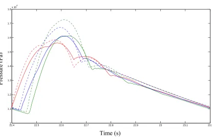
Fig. 4.4 Comparison of pressures for modified resistances.
Red-Inlet, Blue-Midpoint, Green-Outlet; Solid-Simulation, Dashed-Alastruey (2006).
22.4 22.5 22.6 22.7 22.8 22.9 23 23.1 23.2
1 1.1 1.2 1.3 1.4 1.5 1.6 1.7 1.8x 10
4
TIme (s)
P
ressu
re
(
P
a)
Time (s)
Pressure
(Pa
Fig. 4.5 Comparison of flows for modified resistances.
Red-Inlet, Blue-Midpoint, Green-Outlet; Solid-Simulation, Dashed-Alastruey (2006).
We can observe from the graphs that the flow profiles have improved, while the pressure magnitudes continue to be off. However, in this case, the pressure at the outlet is actually greater than that at the midpoint (even though by a very small amount), as is expected physiologically. We can also see that the shape of both, the pressure and flow curves have improved and are now more similar to that of Alastruey. Attempts were made with further decreasing Ru, but the results were not satisfactory. To increase the magnitudes of the pressure curves, the modulus was increased to 4.2x10⁵ Pa, but the results were very similar.
22.4 22.5 22.6 22.7 22.8 22.9 23 23.1 23.2
-0.5 0 0.5 1 1.5 2 2.5 3 3.5x 10
-4
TIme (s)
Fl
o
w
(
m
3
/s
)
Flow
(m
3 /s
)
Thus, the most successful run was the one with the same geometrical and elastic parameters as that of Alastruey, but with a lower Ru and a higher Rd.
4.2.4 Simulation with Bifurcation Conditions
Another simulation was done with the bifurcation model. The inlet flow was the same as that of Alastruey (2006); however, instead of the WK3 model as the outflow BC, we now had a bifurcation condition at the outlet of the aorta, which bifurcated into two arteries. These two daughter vessels had WK3 as the outlet BC (the WK3 parameters were same as used by Alastruey). The results are shown in Fig. (4.6).
Fig. 4.6 Pressure for run with bifurcation conditions. Red-Inlet, Blue-Midpoint,
Green-10.3 10.4 10.5 10.6 10.7 10.8 10.9 11 11.1 11.2 11.3
0.4 0.6 0.8 1 1.2 1.4 1.6
1.8x 10
4
Time (s)
P
res
ure
(
P
a
)
Pressure
(Pa
)
Fig. 4.7 Flow plot for run with bifurcation conditions. Red-Inlet, Blue-Midpoint, Green-Outlet; Solid-Simulation, Dashed-Alastruey (2006).
We notice that the overall trend and the shapes of the pressure and flow plots are the same as that of Alastruey (2006), but the magnitudes are lower. By increasing the elastic modulus to 5.2 x10⁵ Pa (instead of 4 x10⁵ Pa), we obtain the following results given in Figure (4.8).
10.4 10.5 10.6 10.7 10.8 10.9 11 11.1 11.2 11.3 11.4
-0.5 0 0.5 1 1.5 2 2.5 3
3.5x 10
-4
Time (s)
Fl
o
w
(
m
3/
s)
Flow
(m
3 /s
)
Fig. 4.8 Pressure for run with E=5.2 x10⁵ Pa. Red-Inlet, Blue-Midpoint, Green-Outlet; Solid-Simulation, Dashed-Alastruey (2006).
21.5 21.6 21.7 21.8 21.9 22 22.1 22.2 22.3 22.4 22.5
0.4 0.6 0.8 1 1.2 1.4 1.6
1.8x 10
4
Time
P
ressu
re
21.6 21.7 21.8 21.9 22 22.1 22.2 22.3 22.4
-0.5 0 0.5 1 1.5 2 2.5 3
3.5x 10
-4
Time
Fl
o
w
Pressure
(Pa
)
Flow
(m
3 /s
)
Time (s)
We can observe that the difference in magnitudes is much lower in this case than in the previous one. Also, all the physiological trends, like the steepening of the pressure curve and the increase in the peak pressure towards the periphery, are captured. It may seem that further increasing the modulus may eventually match the magnitudes with those of Alastruey, which is not the case. Further increase in the modulus makes the artery behave more like a rigid tube and hence the peak pressure decreases downstream.
Attempts were also made by modifying the WK3 resistances, but the results were very similar. It is expected that the results in this bifurcation model will not be matching because the waveforms in the aorta will depend on the reflected waves form the bifurcation, which in turn depend on the radius and length of the daughter vessels. The fact that the bifurcation BC produces results very similar to those for the WK3 BC validates the bifurcation condition.
Thus, it is clear that the model is able to reproduce all the required trends as that of Alastruey, although some minor modifications in parameters are needed. The differences that are seen are only in the magnitudes and can be caused due to the different methods in applying the WK3 BC. They implement the WK3 model differently than us, taking into account a constant venous pressure while we do not. In the electrical analogy, we have our ‘ground’ as zero pressure while Alastruey have theirs at the venous pressure.
4.3 Validation with Experimental/Computational Observations by Kung et al. (2011)
In this experimental paper, Kung et al. (2011) have compared the simulated results from a 3-D model of a single compliant vessel with experimental data obtained for the same vessel.
4.3.1 The Experiment
4.3.2 The Simulation
Kung et al. (2011) developed a 3-D model of the compliant vessel and adopted the CMM-FSI technique developed by Figueroa et al. (2006). This FSI technique is based on the thin wall approximation and assumes that the walls behave as a linear membrane (i.e. linear elasticity). The physiological input as shown in Figure (4.11) was applied to the inlet while a WK4 model formed the outlet BC. The WK parameters were based on the flow and pressure data acquired from the experiment.
The authors determined a static elastic modulus of 9.1x10⁵ Pa and a dynamic modulus of 1 MPa for the silicone material and an operating radius of 1.13 cm at an operating pressure of 96 mmHg (12798.9 Pa).
Fig. 4.11 Physiological flow input to the model (Kung et al. (2011))
0 0.1 0.2 0.3 0.4 0.5 0.6 0.7 0.8 0.9 1
-4 -2 0 2 4 6 8 10 12
14x 10
-5
Time (s)
Flo
w
(
m
3
/s
)
Time (s)
Flow
(m
3 /s
4.3.3 Parameters Used in Our Model
In order to simulate the physiological input, a Fourier series with eight terms was used to approximate the flow pattern shown in Figure (4.11). For the outlet BC, a WK3 model was used. The parameters used for this WK3 were based on those of WK4 and the outlet flow and pressures as given in Kung et al. (2011). (Values as used in Childress (2013) for the same validation).
Ru=28.4268x10⁶ Pa.s/m3, Rd=384.3939 Pa.s/m3, C=1.384x10⁻⁹ m3/Pa.
The 1-D code was run for the above parameters and the results were compared with those obtained experimentally by Kung et al. (2011):
Fig. 4.12 Pressure plot for E= 1 MPa, r0= 1 cm. Red-Inlet, Blue-Midpoint, Green-Outlet;
11 11.1 11.2 11.3 11.4 11.5 11.6 11.7 11.8 11.9 12
0.9 1 1.1 1.2 1.3 1.4 1.5 1.6 1.7x 10
4
TIme (s)
Pr
e
s
s
u
re
(
P
a)
Time (s)
Pressure
(Pa
Fig. 4.13 Flow plot for E= 1 MPa, r0= 1 cm. Red-Inlet, Blue-Midpoint, Green-Outlet; Solid-Simulation, Dashed- Kung et al. (2011).
The waveform converged by around 7-8 pulses. The time required with 50 grid points was about 25 seconds. We can see that the flow rates match well while the pressures seem a bit lower. As a remedy, it was decided to run the code with a slightly increased modulus, since increasing the modulus stiffens the artery which would increase the pressure. This is because stiffer vessels would have less give, i.e. the flow area would be smaller but flow rates would be same, hence pressures would be higher. The next figures depict the results with a modulus of 1.2 MPa, other parameters being same.
11 11.1 11.2 11.3 11.4 11.5 11.6 11.7 11.8 11.9 12
-4 -2 0 2 4 6 8 10 12 14x 10
-5
Time (s)
Fl
o
w
(
m
3
/s
)
Time (s)
Flow
(m
3 /s
Fig. 4.14 Pressure plot for E= 1.2 MPa, r0= 1 cm. Red-Inlet, Blue-Midpoint, Green-Outlet; Solid-Simulation, Dashed- Kung et al. (2011).
10 10.1 10.2 10.3 10.4 10.5 10.6 10.7 10.8 10.9 11
0.9 1 1.1 1.2 1.3 1.4 1.5 1.6 1.7
1.8x 10
4 Time P re ssu re
10 10.1 10.2 10.3 10.4 10.5 10.6 10.7 10.8 10.9 11
-4 -2 0 2 4 6 8 10 12
14x 10
By comparing these plots with those for E=1MPa, we observe that higher modulus clearly improved the results for both, the pressure and the flow rates. The corresponding wall displacement (change in radius) is indicated in Fig. (4.16).
Fig. 4.16 Change in radius for E= 1.2 MPa, r0= 1 cm. Red-Inlet, Blue-Midpoint, Green-Outlet
The plots for pressure and wall displacement show that the two quantities are proportional, as expected (since we have used an algebraic relation between pressure and area). One more run was done using E=1 MPa and the radius was reduced by 0.0008 m, corresponding to the thickness of the vessel, but it gave very similar results to those for E=1.2 MPa and r0=1 cm. This is because increasing the modulus and decreasing the radius, both make the vessel stiffer.
10 10.1 10.2 10.3 10.4 10.5 10.6 10.7 10.8 10.9 11 0.8
0.9 1 1.1 1.2 1.3 1.4 1.5 1.6x 10
-3
Time (s)
W
a
ll dis
p
la
ce
m
e
n
t (
m
4.4 Validation with the Model by Marchandise et al. (2009)
4.4.1 Model Details
This validation was done primarily to validate the bifurcation boundary conditions. In their article, Marchandise et al. (2009) used a 1-D model to analyze the hemodynamic parameters within arteries and its application to bypass surgery. They use a model similar to that used by Alastruey (2006). Their hyperbolic system of equations was in the A-u form assuming a flat velocity profile.
0 4.11
1
0 4.12
Where K=22πμ. The state equation is the tube law representing relation between the pressure and area as:
, √ 4.13
with
4√
3 4.14
On comparison we find that this is the same pressure area relationship that is used by Alastruey (2006). This system is then discretized using a Discrete Galerkin method and a four stage explicit Runge-Katta scheme.
Following is the visualization of the geometry of the system:
Fig. 4.17 Geometry for validation of the bifurcation.
As is seen from the figure, the parent vessel has a length of 20 cm and a radius of 0.5 cm while the daughters have lengths of 20 cm and radius of 0.2041 cm each. The radii of the daughters are selected so as to get a reflection coefficient of 0.5 for the bifurcation (Sherwin et al. (2003)). This would mean that at the bifurcation, the magnitude of the reflected wave would be half of that of the incident wave. Also, for this case, the viscosity was set to zero to simplify the case.
4.4.2 Boundary Conditions
At the inlet, the inflow velocity is specified. The inflow velocity is transient and is in the form of a Gaussian bell curve:
0, 0.5 5000 0.05 4.15
For the bifurcation boundary condition, the authors enforced conservation of mass and balance of energy at the bifurcation interface to get the flow variables for the parent and the daughters.
L=20 cm, r0 =0.5cm
L=20 cm, r0 =0.2041cm
At the outlet, the authors apply an absorbing boundary condition which means that there is no reflection form the outlet boundary.
4.4.3 Implementation
The elasticity for all the vessels is specified in terms of the parameter β. β=32.497 cm-2 g s-2 for the parent and β=79.692 cm-2 g s-2 for the daughters. From these values and Equation (4.14) for β, we can find out the value of the parameter Eh/r0 to be substituted in
our model. The geometry of the vessels was kept the same as that given in the article.
The inflow boundary condition was specified as the inlet flow rate by multiplying the given inlet velocity expression with the inlet area. The bifurcation conditions were the same as were coded before and for the absorbing outlet boundary conditions, the values of the flow variables at the outlet grid point were kept equal to those at the grid point before it at the previous time step.
4.4.4 Results
Fig. 4.18 Pressure plots from 1-D and those of Marchandise et al. (2009).
It is seen from the pressure plots that our results match those of Marchandise et al. (2009) well. The blue curve shows the pressure variation in time at the inlet. Thus, we see that the pressure wave travels from the inlet to the midpoint of the parent vessel (green) and then to the outlet of the parent vessel (red). At the outlet, the incident pressure wave which has magnitude of about 60 dynes/cm2 is reflected. Also, at the bifurcation, the reflected and incident waves coincide increasing the resultant pressure. This stepped up pressure wave then travels through the daughter vessels (cyan-midpoint and violet-outlet). At the same time, the reflected wave (from the bifurcation) travels backwards towards the inlet of the parent vessel and reaches the midpoint and then finally the inlet of the parent vessel. We see that the
0 0.05 0.1 0.15 0.2 0.25 0.3 0.35 0.4 0.45 0.5
-10 0 10 20 30 40 50 60 70 80 90 Time (s) P ress u re ( dyne /c m 2 ) Inlet Midpoint Outlet D-Midpoint D-Outlet
Inlet-Marchandise et al. Midpoint-Marchandise et al. Outlet-Marchandise et al. D-Midpoint-Marchandise et al. D-Outlet-Marchandise et al.
Time (s)
Pressure
(Pa