ABSTRACT
BHAUMIK, PRITHWISH. Bayesian Estimation and Uncertainty Quantification in Differential Equation Models. (Under the direction of Subhashis Ghoshal.)
In engineering, physics, biomedical sciences, pharmacokinetics and pharmacodynam-ics (PKPD) and many other fields the regression function is often specified as solution of a system of ordinary differential equations (ODEs) given by
dfθ(t)
dt =F(t,fθ(t),θ), t ∈[0,1];
here F is a known appropriately smooth vector valued function. Our interest lies in es-timating θ from the noisy data.
A two-step approach to solve this problem consists of the first step fitting the data nonparametrically, and the second step estimating the parameter by minimizing the dis-tance between the nonparametrically estimated derivative and the derivative suggested by the system of ODEs. In Chapter 2 we consider a Bayesian analog of the two step ap-proach by putting a finite random series prior on the regression function using B-spline basis. We establish a Bernstein-von Mises theorem for the posterior distribution of the parameter of interest induced from that on the regression function with the n−1/2 con-traction rate.
Although this approach is computationally fast, the Bayes estimator is not asymp-totically efficient. This can be remedied by directly considering the distance between the function in the nonparametric model and a Runge-Kutta (RK4) approximate solution of the ODE while inducing the posterior distribution on the parameter as done in Chapter 3. We also study the asymptotic properties of a direct Bayesian method obtained from the approximate likelihood obtained by the RK4 method in Chapter 3.
Chapters 4 and 5 contain the extensions of the methods discussed so far for higher order ODE’s and partial differential equations (PDE’s) respectively.
Bayesian Estimation and Uncertainty Quantification in Differential Equation Models
by
Prithwish Bhaumik
A dissertation submitted to the Graduate Faculty of North Carolina State University
in partial fulfillment of the requirements for the Degree of
Doctor of Philosophy
Statistics
Raleigh, North Carolina 2015
APPROVED BY:
Soumendra Nath Lahiri Alyson Wilson
Yichao Wu Subhashis Ghoshal
DEDICATION
BIOGRAPHY
ACKNOWLEDGEMENTS
I would like to thank my advisor Dr. Subhashis Ghoshal for guiding me to lay the foun-dation of my research career. His constant help has made it possible for me to finish my doctoral work in a proper and timely fashion. I would also like to express my sincere gratitude to Dr. Soumendra Nath Lahiri, Dr. Alyson Wilson and Dr. Yichao Wu for agreeing to be in my graduate advisory committee.
The Statistics department of North Carolina State university has provided me with all the kinds of help a graduate student can look for. The faculty members have been extremely helpful and easily approachable. I would specifically mention Dr. Sujit Ghosh, Dr. Donald Martin and Dr. Arnab Maity in this regard. I have also received a lot of help from the department staff members. I am extremely grateful to Alison McCoy and Terry Byron who have always answered all my queries with a smiling face.
My four years of stay in the USA has been a memorable chapter of my life. I have been fortunate enough to have a wonderful group of friends including Souvik Chandra, Sayantan Banerjee, Ayan Das Gupta, Shuva Gupta, Lopamudra Kundu, Ritwik Chat-terjee, Saswata Sahoo, Priyam Das, Debraj Das, Arnab Hazra, Arkaprava Roy, Indrani Sahoo, Moumita Chakraborty and Sohini Raha.
TABLE OF CONTENTS
LIST OF TABLES . . . vii
LIST OF FIGURES . . . viii
LIST OF SYMBOLS . . . ix
Chapter 1 Introduction . . . 1
1.1 Literature review . . . 4
1.1.1 Non-linear least squares approach . . . 4
1.1.2 Generalized profiling approach . . . 5
1.1.3 Multiple shooting approach . . . 5
1.1.4 Two-step approach . . . 6
1.1.5 Bayesian estimation techniques . . . 7
1.1.6 Parameter estimation for higher order ODE model . . . 7
1.1.7 Parameter estimation for PDE model . . . 8
1.2 Contributions of the thesis . . . 8
Chapter 2 Bayesian two-step procedure based on splines . . . 10
2.1 Introduction . . . 10
2.2 Model assumption and prior specification . . . 11
2.3 Main results . . . 13
2.4 Extensions . . . 16
2.5 Simulation Study . . . 18
2.6 Real life data . . . 19
2.7 Proofs of theorems . . . 21
2.8 Proofs of the lemmas . . . 31
Chapter 3 Bayesian methods based on Runge-Kutta approximation . . 39
3.1 Introduction . . . 39
3.2 Preliminaries of Runge-Kutta method . . . 40
3.3 Model assumptions and prior specifications . . . 41
3.3.1 Runge-Kutta Sieve Bayesian Method (RKSB) . . . 42
3.3.2 Runge-Kutta Two-step Bayesian Method (RKTB) . . . 43
3.4 Main results . . . 43
3.5 Simulation Study . . . 45
3.6 Proofs . . . 46
3.7 Proofs of the lemmas . . . 50
equa-4.1 Introduction . . . 68
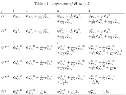
4.2 Preliminaries of Runge-Kutta method for higher order ODE . . . 69
4.3 Model description and prior specification . . . 72
4.4 Methodology . . . 72
4.4.1 Runge-Kutta Sieve Bayesian Method (RKSB) . . . 73
4.4.2 Runge-Kutta Two-step Bayesian Method (RKTB) . . . 74
4.4.3 Two-step Bayesian Method . . . 75
4.5 Main results . . . 75
4.6 Simulation Study . . . 78
4.7 Proofs . . . 79
Chapter 5 Bayesian inference for partial differential equation models . 84 5.1 Introduction . . . 84
5.2 Model description and prior specification . . . 85
5.3 Results . . . 87
5.4 Simulation Study . . . 88
5.5 Proofs . . . 89
Chapter 6 Future directions . . . 95
6.1 Efficient Bayesian inference for partial differential equation models using numerical solution . . . 95
6.1.1 Parabolic Equation . . . 95
6.1.2 Hyperbolic Equation . . . 96
6.1.3 Elliptic Equation . . . 96
6.2 Bayesian uncertainty quantification for non-add-itive error . . . 97
References . . . 99
Appendix . . . 104
LIST OF TABLES
Table 2.1 Coverages and average lengths of the Bayesian credible interval and confidence interval obtained from VB method . . . 19 Table 3.1 Coverages and average lengths of the Bayesian credible intervals for the
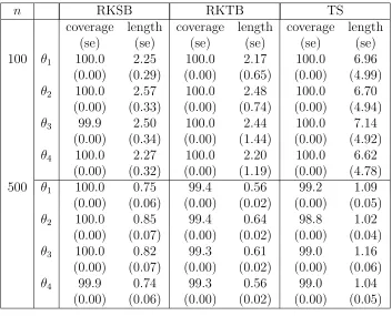
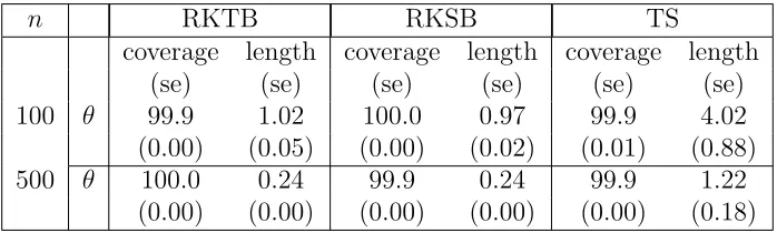
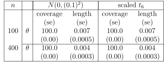
three methods . . . 47 Table 4.1 Arguments of H in (4.2) . . . 71 Table 4.2 Coverages and average lengths of the Bayesian credible intervals for the
LIST OF FIGURES
Figure 1.1 Logarithm of growth over time of the three colonies . . . 2 Figure 1.2 Prey and predator population following the Lotka-Volterra equations . 3 Figure 2.1 Observed values and the posterior predictive intervals for the three
LIST OF SYMBOLS
:= equality by definition.
((Ai,j)) : a matrix A with (i, j)th element being Ai,j. AT : transpose of the matrix A.
Ai,: the ith row ofA. A,j : the jth column of A.
rowssr(A) : the sub-matrix of A consisting of rth tosth rows ofA with r < s. colssr(A) : the sub-matrix of Aconsisting of rth to sth columns ofAwith r < s. xr:s : the sub-vector consisting of rth tosth elements of a vector x.
vec(A) : the vector obtained by stacking the columns of the matrixAone over another.
A⊗B: the Kronecker product between Aand B.
Ip : the identity matrix of order p.
maxeig(A) : the maximum eigenvalue of the matrix A. mineig(A) : the minimum eigenvalue of the matrix A. kxk: (Pp
i=1x 2
i)
1/2
, the L2 norm of the vector x. f0(t) : dtdf(t), the derivative of the function f(·). f(r)(t) : dr
dtrf(t), the rth order derivative of the function f(·).
f(·) : a vector valued function.
kfkw : (R01kf(t)k2w(t)dt)1/2 for functions f : [0,1]→
Rp and w: [0,1]→[0,∞).
f(x) : (f(x1), . . . , f(xp))T for a real-valued function f : [0,1]→R and a vector x∈Rp.
h·,·i: inner product. l
1A(·) : indicator function of the set A.
an =o(bn) : an/bn→0 as n → ∞ for numerical sequences an and bn.
an =O(bn) :an/bn is bounded.
an bn: an =O(bn) and bn =O(an).
an .bn: an =O(bn).
an bn: bn=o(an).
an bn: an =o(bn).
oP(1) : a sequence of random variables which converges in probability to zero.
OP(1) : a sequence of random variables bounded in probability. E(·) : the mean vector of a random vector.
kP −QkT V : supB∈Rp|P(B)−Q(B)|, the total variation distance between P and Q. Cm(E) : the collection of functions defined on an open set E with first m continuous
partial derivatives with respect to its arguments. ˙
fθ(x) : ∂θ∂ fθ(x) for the functionθ 7→fθ(x).
¨
fθ(x) : ∂
2
∂θ2fθ(x) for the functionθ 7→fθ(x).
Pnψ :n−1
Pn
i=1ψ(Xi) for a sample {Xi : i= 1, . . . , n} and a measurable function ψ(·).
Gnψ :
√
n(Pnψ−Eψ).
a∧b : the minimum of two real numbersa and b. Drf(t) : ∂t∂rr1+1···+rs
1 ···∂t rs
s f(t) for a vectorr = (r1, . . . , rs)
T of nonnegative integers and a function
f :Rs 7→
R.
|r|:Ps
j=1rj for a vector r = (r1, . . . , rs)
Chapter 1
Introduction
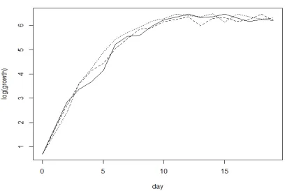
Differential equations are encountered in various branches of science such as in genetics (Chen et al., 1999), viral dynamics of infectious diseases [Anderson and May (1992), Nowak and May (2000)]. Diggle (1990) contains a data set on the growth of three closed colonies of paramecium aurelium in a nutritive medium over a period of 19 days. The logarithm of the growth for the three colonies are plotted in Figure 1.1. Denoting byµ(t) as the logarithm of growth at time t, Ghosh and Goyal (2010) suggested the possible ordinary differential equation (ODE) model as
dµ(t)
dt = θ1−θ2exp{µ(t)}, µ(0) = log 2.
There are numerous applications in the fields of pharmacokinetics and pharmacodynamics (PKPD) as well. There are a lot of instances where no closed form solution exist. Such an example can be found in the feedback system (Gabrielsson and Weiner, 2006, page 332) modeled by the ODEs
dR(t)
dt =
kin
M(t) −koutR(t), dM(t)
Figure 1.1: Logarithm of growth over time of the three colonies
where R(t) and M(t) stand for loss of response and modulator at time t respectively. Herekin, kout andktolare unknown parameters which have to be estimated from the noisy observations. Another popular example is the Lotka-Volterra equations, also known as predator-prey equations. At time t ∈ [0,1] the prey and predator populations change according to the equations
df1θ(t)
dt = θ1f1θ(t)−θ2f1θ(t)f2θ(t), df2θ(t)
dt = −θ3f2θ(t) +θ4f1θ(t)f2θ(t),
whereθ= (θ1, θ2, θ3, θ4)T andf1θ(t) andf2θ(t) denote the prey and predator populations
at timetrespectively. A noisy data from this model is shown in Figure 1.2. These models can be put in a regression model
Yi =fθ(ti) +εi, (1.1)
for i= 1, . . . , n with θ ∈Θ⊆Rp and f
θ : [0,1]7→Rd and fθ(·) satisfies the ODE
dfθ(t)
Figure 1.2: Prey and predator population following the Lotka-Volterra equations
here F is a known appropriately smooth vector valued function and θ is a parameter vector controlling the regression function.
Some physical events can be described using higher order ODE’s. Let G(t) and H(t) respectively be the concentrations of glucose and hormone in blood at timet. Denoting by G0(t) andH0(t) the corresponding optimal values at timet, we are interested in studying the behavior of g(t) = G(t)−G0(t) and h(t) = H(t)−H0(t). These quantities change according to the system of ODE’s
dg(t)
dt = −m1g(t)−m2h(t) +J(t), dh(t)
dt = −m3h(t) +m4g(t),
J(t) being a known function denoting the external rate of increase of blood glucose con-centration. Here m1, m2, m3 and m4 are unknown parameters. Since we cannot measure h(t), the two equations are combined to get the second order ODE
d2g(t) dt2 + 2α
dg(t) dt +ω
2
whereα = (m1+m3)/2, ω20 =m1m3+m2m4 and S(t) =m3J(t) +J0(t). More generally, we often come across higher order ODE models of the form
F t,fθ(t),f
(1)
θ (t), . . . ,f
(q)
θ (t),θ
=0, (1.3)
F being a known sufficiently smooth vector valued function.
There are also instances when we encounter partial differential equation (PDE) mod-els. For example Xun et al. (2013) addressed a problem using the PDE model
∂g(t, z) ∂t −θD
∂2g(t, z) ∂z2 −θS
∂g(t, z)
∂z −θAg(t, z) = 0
where g(t, z) is the signal over time t and range z and θA,θD and θS are the parameters
of interest. Formally speaking, the regression function is governed by the αth order PDE
F (t,(Drfθ :|r| ≤α),θ) = 0, F being known and t = (t1, . . . , ts)T.
1.1
Literature review
There have been a significant number of works done on parameter estimation in the past few decades. We present them below.
1.1.1
Non-linear least squares approach
If the ODEs can be solved analytically, then the usual non linear least squares (NLS) [Levenberg (1944), Marquardt (1963)] can be used to estimate the unknown parameters. Thus
ˆ
θ = arg min
θ∈Θ
n
X
i=1
In many contexts, such closed form solutions are not available as evidenced in some of the previous examples. Hairer et al. (1987) and Mattheij and Molenaar (1996) used the 4-stage Runge-Kutta algorithm as an alternative approach. The statistical properties of the corresponding estimator have been studied by Xue et al. (2010). The strong consistency, √
n-consistency and asymptotic normality of the estimator were established in their work.
1.1.2
Generalized profiling approach
Ramsay et al. (2007) proposed the generalized profiling procedure where the solution is approximated by a linear combination of basis functions given byf(·) = βTφ, whereβis the vector of coefficients. The coefficients of the basis functions are estimated by solving a penalized optimization problem using an initial choice of the parameters of interest. A data-dependent fitting criterion Hn(f) and a penalty termJ(f,θ) are constructed. For
a givenθ they define ˆ
β(θ) = arg max
β Hn(β
Tφ)−λJ(βTφ,θ)
,
λ being a tuning parameter. Then the parameter estimate is obtained as ˆ
θ= arg max
θ∈Θ Hn(β
T(θ)φ)
.
Qi and Zhao (2010) explored the statistical properties of this estimator including √ n-consistency and asymptotic normality. Despite having desirable statistical properties, these approaches are computationally cumbersome especially for high-dimensional sys-tems of ODEs as well as whenθ is high-dimensional.
1.1.3
Multiple shooting approach
Baake et al. (1992) viewed the ODE as a multi-point boundary value problem by dividing [0,1] into a grid of multiple shooting nodes 0 =τ0 < τ1 < τ2 <· · ·< τm < τm+1 = 1 and considering the initial value problems
for j = 1, . . . , m+ 1. Here s1, . . . , sm+1 are also treated as unknown parameters and the new parameter vector (s1, . . . , sm+1,θ)T is estimated using least squares technique subject to the constraints (1.4). Naturally this method will give a solution with discontinuous trajectory which can be made continuous by introducing additional continuity criteria. This method also has high computational cost.
1.1.4
Two-step approach
Varah (1982) used an approach of two-step procedure. In the first step each of the state variables is approximated by a cubic spline using the least squares technique. Let us denote the approximation by ˆf(·). In the second step, the parameter is estimated as
ˆ
θ= arg min
θ∈Θ
n
X
i=1
ˆ
f0(x
i)−F(xi,fˆ(xi),θ)
2 .
This method does not depend on the initial or boundary conditions of the state variables and is computationally very efficient. An example given in Voit and Almeida (2004) showed the computational superiority of the two-step approach over the usual least squares technique. Brunel (2008) replaced the sum of squares of the second step by a weighted integral of the squared deviation, that is
ˆ
θ= arg min
θ∈Θ Z 1
0
ˆ
f0(t)−F(x
i,fˆ(t),θ)
2
w(t)dt
normality of the estimator were also established in their work.
1.1.5
Bayesian estimation techniques
In ODE models Bayesian estimation was considered in the works of Gelman et al. (1996), Rogers et al. (2007) and Girolami (2008). First they solved the ODEs numerically to approximate the expected response and hence constructed the likelihood. A prior was assigned on θ and MCMC technique was used to generate samples from the posterior. Computational cost might be an issue in this case as well.
Campbell and Steele (2012) proposed the smooth functional tempering approach which is a population MCMC technique and it utilizes the generalized profiling approach (Ramsay et al., 2007) and the parallel tempering algorithm. Campbell (2007) and Jaeger et al. (2012) also used a Bayesian analog of the generalized profiling by putting prior on the coefficients of the basis functions.
Chkrebtii et al. (2013) divided the time range into discrete grid points. They put a Gaussian process prior on the solution of the ODE and its derivative. The posterior distribution of the solution is used to draw the posterior sample of the parameter of interest. This method is computationally expensive and the likelihood is required to be known for this approach. The theoretical aspects of Bayesian estimation methods have not been yet explored in the literature.
1.1.6
Parameter estimation for higher order ODE model
The approach has been extended for the case of open higher order ODE’s in Bergstrom (1986).
1.1.7
Parameter estimation for PDE model
M¨uller and Timmer (2002) used the multiple shooting approach for PDE models. A two step approach similar to Varah (1982) using splines was applied by M¨uller and Timmer (2004) to estimate the parameters. Xun et al. (2013) used a parameter cascading method which is a two-step optimization procedure. In the first step a nonparametric B-spline model is fit using penalized least squares approach. The optimal coefficients of the basis functions are expressed as a function of the parameter vector. The second step involves estimating the parameter by least squares method. They established asymptotic normality of the estimator with n−1/2 rate of convergence. In the Bayesian framework, the Bayesian P-splines approach has been used by Xun et al. (2013).
1.2
Contributions of the thesis
In Chapter 2 we consider a Bayesian analog of the approach of Brunel (2008) fitting a nonparametric regression model using B-spline basis. We assign priors on the coefficients of the basis functions. A posterior is induced on θ from the joint posterior of the coef-ficients of the basis functions. In this chapter we study the asymptotic properties of the posterior distribution of θ and establish a Bernstein-von Mises theorem with the n−1/2 contraction rate. Normal distribution is used as the working model for error distribution, but the true distribution of errors may be different. Interestingly, the original model is parametric but it is embedded in a nonparametric model, which is further approximated by high dimensional parametric models. Note that the slow rate of nonparametric estima-tion does not influence the convergence rate of the parameter in the original parametric model.
the posterior of θ using an approximate likelihood function constructed using the nu-merical solution. We call this method Runge-Kutta sieve Bayesian (RKSB) method. In the second approach we define θ as the minimizer of a weighted distance between the function in the nonparametric model and the RK4 numerical solution. We call this ap-proach Runge-Kutta two-step Bayesian (RKTB) method. Thus, this apap-proach is similar in spirit to the two-step Bayesian approach. A prior is assigned on the coefficients of the B-spline basis and the posterior ofθ is induced from the posterior of the coefficients. But the main difference lies in the way of extending the definition of parameter. Instead of using deviation from the ODE, we consider the distance between function in the non-parametric model and RK4 approximation of the model. Both RKSB and RKTB lead to Bernstein-von Mises Theorem with dispersion matrix inverse of Fisher information and hence both the Bayesian methods are asymptotically efficient. This is not the case for the two step-Bayesian approach described in Chapter 2. Bernstein-von Mises Theo-rem implies that credible intervals have asymptotically correct frequentist coverage. The computation cost of the two-step Bayesian method is the least. RKTB is more expensive and RKSB is even more expensive from computational point of view. RKTB is better than other highly computationally intensive Bayesian approaches based on MCMC and Gaussian process prior.
In Chapters 4 and 5 we extend these ideas for higher order ODE models and PDE models. Here the weight function used for two-step approach has to satisfy some addi-tional criteria.
Chapter 2
Bayesian two-step procedure based
on splines
2.1
Introduction
The two step method introduced by Varah (1982) is computationally quite efficient as shown through an example given in Voit and Almeida (2004). Brunel (2008) used a weighted integral of the squared deviation instead of the sum of squares in the second step and proved the asymptotic normality of the estimator with n−1/2 convergence rate. The degree of smoothness of F(·,·,·) with respect to its first two arguments determines the order of the B-spline basis
In this chapter we consider a Bayesian analog of the approach of Brunel (2008). We put a prior on the coefficient vector of the spline based regression model. The Gaussian distribution is used as the working model for error although the true distribution may be different. We also let the ODE model to be misspecified, that is, the true regression function may not be a solution of the ODE. The response variable is also allowed to be multidimensional with possibly correlated errors. A posterior is induced on the parameter of interest from the posterior of the coefficient vector. A Bernstein-von Mises theorem is established for the posterior distribution ofθ with the n−1/2 contraction rate.
We extend the results to more generalized setups in Section 2.4. In Section 2.5 we have carried out a simulation study under different settings. Section 2.6 contains the analysis of a real life data. The proofs of the main results are given in Section 2.7. The Section 2.8 contains the proofs of the required lemmas.
2.2
Model assumption and prior specification
We have a system of d ordinary differential equations given by dfjθ(t)
dt =Fj(t,fθ(t),θ), t ∈[0,1], j = 1, . . . , d, (2.1) where fθ(·) = (f1θ(·), . . . , fdθ(·))T and θ ∈ Θ, where we assume that Θ is a compact
subset of Rp. Let us denote F(·,·,·) = (F1(·,·,·), . . . , Fd(·,·,·))T. We also assume that
for a fixed θ, F ∈ Cm−1((0,1),Rd) for some integer m ≥ 1. Then, by successive differ-entiation of the right hand side of (2.1), it follows that fθ ∈ Cm((0,1)). By the implied
uniform continuity, the function and its several derivatives uniquely extend to continuous functions on [0,1].
Consider an n × d matrix of observations Y with Yi,j denoting the measurement
taken on thejthresponse at the pointx
i, 0≤xi ≤1, i= 1, . . . , n; j = 1, . . . , d. Denoting ε= ((εi,j)) as the corresponding matrix of errors, the proposed model is given by
Yi,j =fjθ(xi) +εi,j, i= 1, . . . , n, j = 1, . . . , d, (2.2)
while the data is generated by the model
Yi,j =fj0(xi) +εi,j, i= 1, . . . , n, j = 1, . . . , d, (2.3)
wheref0(·) = (f10(·), . . . , fd0(·))T denotes the true mean vector which does not necessarily belong to {fθ : θ ∈ Θ}. We assume that f0 ∈ Cm([0,1]). Let εi,j
iid
∼ P0, which is a probability distribution with mean zero and finite variance σ2
0 for i = 1, . . . , n;j = 1, . . . , d.
in the nonparametric regression model
Y =XnBn+ε, (2.4)
whereXn= ((Nj(xi)))1≤i≤n,1≤j≤kn+m−1,{Nj(·)}kj=1n+m−1 being the B-spline basis functions of order m with kn−1 interior knots. Here we denote
Bn=
β(1kn+m−1)×1, . . . ,β(dkn+m−1)×1,
the matrix containing the coefficients of the basis functions. Also we consider P0 to be unknown and use N(0, σ2) as the working distribution for the error where σ may be treated as another unknown parameter. Let us denote by t1, . . . , tkn−1 the set of interior knots with tl =l/kn for l = 1, . . . , kn−1. Hence the meshwidth is ξn = 1/kn. Denoting
byQn, the empirical distribution function ofxi, i= 1, . . . , n, we assume
sup
t∈[0,1]
|Qn(t)−Q(t)|=o(kn−1)
for some distribution functionQ(·) with positive continuous density. Let the prior distri-bution on the coefficients be given by
βj iid
∼Nkn+m−1(0, nc−1k−1n (X T
nXn)−1) (2.5)
for some constant c >0. Simple calculation yields the posterior distribution for βj as βj|Y ∼Nkn+m−1
c−1n (XnTXn)
−1
XnTY,j, c−1n σ
2(XT
nXn)−1
(2.6) and the posterior distributions ofβj and βj0 are mutually independent for j 6=j0; j, j0 =
1, . . . , d, where cn = (1 +σ2ckn/n). By model (2.4), the expected response vector at a
point t∈[0,1] is given byBT
nN(t), where N(·) = (N1(·), . . . , Nkn+m−1(·))T.
(0,1). We define
Rf(η) =
Z 1
0
kf0(t)−F(t,f(t),η)k2w(t)dt
1/2
,
ψ(f) = arg min
η∈ΘRf(η). (2.7)
It is easy to check that ψ(fη) =η for all η∈Θ. Thus the map ψ extends the definition
of the parameter θ beyond the model. Let us define θ0 = ψ(f0). We assume that θ0 lies in the interior of Θ. From now on, we shall write θ for ψ(f) and treat it as the parameter of interest. A posterior is induced on Θ through the mapping ψ acting on
f(·) =BT
nN(·) and the posterior ofBn given by (2.6).
2.3
Main results
Our objective is to study the asymptotic behavior of the posterior distribution of√n(θ−
θ0). The asymptotic representation of √
n(θ−θ0) is given by the next theorem under the assumption that
for all >0, inf
η:kη−θ0k≥
Rf0(η)> Rf0(θ0). (2.8)
We denote Dl,r,sF(t,f,θ) = ∂l+r+s/∂θs∂fr∂tlF(t,f(t),θ). Since the posterior
distribu-tions ofβj are mutually independent whenε,j are mutually independent forj = 1, . . . , d,
we can assume d = 1 in Theorem 2.1 for the sake of simplicity in notation and write f(·), f0(·), F(·,·,·), β instead of f(·), f0(·), F(·,·,·) and Bn respectively. Extension to
d-dimensional case is straightforward as shown in Remark 2.5 after the statement of Theorem 2.1. We deal with the situation of correlated errors in Section 2.4.
Theorem 2.1. Let the matrix
J(θ0) =
Z 1
0
(D0,0,1F(t, f0(t),θ0))TD0,0,1F(t, f0(t),θ0)w(t)dt
−
Z 1
be nonsingular, where
S(t, f(t),θ) = (D0,0,1F(t, f(t),θ))T(f00(t)−F(t, f0(t),θ0)).
Let m be an integer greater than or equal to 5 andn1/2m k
nn1/8. IfD0,2,1F(t, y,θ)
and D0,0,2F(t, y,θ) are continuous in their arguments, then under the assumption (2.8),
there existsEn ⊆Cm((0,1))×ΘwithΠ(Enc|Y) =oP0(1), such that uniformly for(f,θ)∈ En,
√
n(θ−θ0)−(J(θ0)) −1√
n(Γ(f)−Γ(f0))
→0 (2.9)
as n → ∞, where
Γ(z) =
Z 1
0
−(D0,0,1F(t, f0(t),θ0))TD0,1,0F(t, f0(t),θ0)w(t) −d
dt[(D0,0,1F(t, f0(t),θ0))
Tw(t)] + (D
0,1,0S(t, f0(t),θ0))w(t)
z(t)dt.
Remark 2.2. Condition (2.8) implies that θ0 is the unique point of minimum of Rf0(·) and θ0 should be a well-separated point of minimum.
Remark 2.3. The posterior distribution ofΓ(f)−Γ(f0) contracts at0at the raten−1/2 as indicated by Lemma 2.14. Hence, the posterior distribution of (θ−θ0) contracts at 0
at the rate n−1/2 with high probability under the truth. We refer to Theorem 2.6 for a more refined version of this result.
Remark 2.4. We note that at least fifth order smoothness of the true mean function is sufficient to ensure the contraction rate n−1/2. We do not gain anything more by assuming a higher order of smoothness. For m = 5, the required condition becomes n1/10 kn n1/8. Also, the knots are chosen deterministically and there is no need
to assign a prior on the number of terms of the random series used. Hence, the issue of Bayesian adaptation, that is, improving convergence rate with higher smoothness without knowing the smoothness, does not arise in the present context.
matrix
(J(θ0)) −1
{−(D0,0,1F(t,f0(t),θ0))TD0,1,0F(t,f0(t),θ0)w(t) −d
dt[(D0,0,1F(t,f0(t),θ0))
Tw(t)] + (D
0,1,0S(t,f0(t),θ0))w(t)}. Then we have
(J(θ0)) −1
Γ(f) =
d
X
j=1
Z 1
0
A,j(t)NT(t)βjdt= d
X
j=1
GTn,jβj, (2.10)
where GT n,j =
R1
0 A,j(t)N
T(t)dt which is a p×(k
n+m−1) matrix forj = 1, . . . , d.
Thus in order to approximate the posterior distribution of θ, it suffices to study the asymptotic posterior distribution of the linear combination of βj given by (2.10). The next theorem describes the approximate posterior distribution of √n(θ−θ0).
Theorem 2.6. Define
µn = √n
d
X
j=1
Gn,jT (XnTXn)−1XnTY,j−√n(J(θ0)) −1
Γ(f0),
Σn = n d
X
j=1
GTn,j(XnTXn)−1Gn,j
and Bj = ((hAk,j(·), Ak0,j(·)i))
k,k0=1,...,p for j = 1, . . . , d. If Bj is non-singular for all
j = 1, . . . , d, then under the conditions of Theorem 2.1,
Π
√
n(θ−θ0)∈ ·|Y
−N µn, σ2Σn
assures that putting a prior on σ rectifies the problem.
Theorem 2.7. We assign independent N(0, nc−1kn−1σ2(XT
nXn)−1) prior on βj for j =
1, . . . , d and a constant c > 0 and inverse gamma prior on σ2 with shape and scale parameters a and b respectively. If the fourth order moment of the true error distribution is finite, then under the conditions of Theorems 2.1 and 2.6
Π
√
n(θ−θ0)∈ ·|Y
−N µn, σ20Σn
T V =oP0(1). (2.12)
2.4
Extensions
The results obtained so far can be extended for the case whereεi,j andεi,j0 are associated
for i = 1, . . . , n and j 6= j0;j, j0 = 1, . . . , d. Let under the working model, εi, have the
dispersion matrix Σ =σ2Ω for i = 1, . . . , n, Ω being a known positive definite matrix. Denoting Ω−1/2 = ((ωjk))d
j,k=1, we have the following extension of Theorem 2.6.
Theorem 2.8. Define
µ∗n = √n
d
X
k=1
colsk(k(k−1)(n+mkn+−1)m−1)+1 GTn,1. . .GTn,d
Ω1/2⊗Ikn+m−1
×(XnTXn)
−1
XnT d
X
j=1
Y,jωjk−
√
n(J(θ0)) −1
Γ(f0),
Σ∗n = n
d
X
k=1
colsk(k(k−1)(n+mkn+−1)m−1)+1 Gn,T1. . .GTn,d Ω1/2⊗Ikn+m−1
×(XnTXn)
−1
×rowsk(k(k−1)(n+mkn+−1)m−1)+1 Ω1/2⊗Ikn+m−1
GTn,1. . .GTn,dT.
Then under the conditions of Theorems 2.1 and 2.6,
Π
√
n(θ−θ0)∈ ·|Y
−N µ∗n, σ2Σ∗n
T V =oP0(1). (2.13)
Theorems 2.1 and 2.7,
Π
√
n(θ−θ0)∈ ·|Y
−N µ∗n, σ20Σ∗n
T V =oP0(1), (2.14)
where σ2
0 is the true value ofσ2.
Remark 2.9. In many applications, the regression function is modeled as hθ(t) = g(fθ(t)) instead of fθ(t), where g is a known invertible function and hθ(t) ∈ Rd. It
should be noted that
dhθ(t)
dt = g
0
(fθ(t))
dfθ(t)
dt
= g0(g−1hθ(t))F(t,g−1hθ(t),θ) = H(t,hθ(t),θ),
which is a known function of t,hθ and θ. Now we can carry out our analysis replacing F and fθ in (1.2) by H and hθ respectively.
Remark 2.10. Often we do not have the data on all the state variables. For the sake of simplicity let d= 2. Let the true regression function be (f1θ0(·), f2θ0(·))
T and suppose
that only the first componentY1 of the response variableY is observable. Let the system of ODE be given by
d
dtf1θ(t) = F1(t, f1θ(t), f2θ(t),θ) (2.15) d
dtf2θ(t) = F2(t, f1θ(t), f2θ(t),θ). (2.16) Model f1(·) by a spline series βTN(·), where β is a free parameter. We substitute this expression for f1(·) and apply the four stage Runge-Kutta method on (2.16) with n grid points to obtain the corresponding nonparametric regression model for Y2 ont given by f2(t) =φn(t, f1(t),θ). Now we define
θ = arg min
η∈Θ Z 1
0
(f10(t)−F1(t, f1(t), f2(t),η)) 2
Then the posterior distribution ofθ induced from that off1(·) will satisfy the Bernstein-von Mises theorem withn−1/2 rate of contraction towardsθ
0. The proof of this assertion is given later.
2.5
Simulation Study
We consider the Lotka-Volterra equations to study the posterior distribution of θ. For a sample of size n, thexi’s are chosen as xi = (2i−1)/2n for i= 1, . . . , n. Samples of sizes
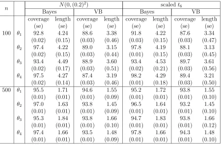
100 and 500 are considered. The weight function is chosen as w(t) = t(1−t), t ∈ [0,1]. We simulate 1000 replications for each case. Under each replication a sample of size 1000 is directly drawn from the posterior distribution of θ and then 95% equal tailed credible interval is obtained. Each replication took around one minute. We calculate the coverage and the average length of the corresponding credible interval over these 1000 replications. The estimated standard errors of the interval length and coverage are given inside the parentheses in the tables. We also consider 1000 replications to construct the 95% equal tailed confidence interval based on asymptotic normality as obtained from the estimation method introduced by Varah (1982) and modified and studied by Brunel (2008). We abbreviate this method by “VB” in tables. The estimated standard errors of the interval length and coverage are given inside the parentheses in the tables. Thus we havep= 4, d= 2 and the ODE’s are given by
F1(t,fθ(t),θ) = θ1f1θ(t)−θ2f1θ(t)f2θ(t),
F2(t,fθ(t),θ) = −θ3f2θ(t) +θ4f1θ(t)f2θ(t)
for t ∈ [0,1] with initial condition f1θ(0) = 1, f2θ(0) = 0.5. The above system is not
analytically solvable. The true mean vector is given by (f1θ0(t), f2θ0(t))
T
, where θ0 = (θ10, θ20, θ30, θ40)T. We take θ10 = θ20 = θ30 = θ40 = 10 to be the true value of the parameter.
and dispersion matrix nc−1kn−1σ2(XT
nXn)−1 with c = 3.5. We choose m = 5. As far as
choosing kn is concerned, we take kn = 17,20 for n = 100 and 500 respectively. The
simulation results are summarized in the Table 2.1. It is clear that both methods give more accurate results as we go on increasing sample size.
Table 2.1: Coverages and average lengths of the Bayesian credible interval and confidence interval obtained from VB method
n N(0,(0.2)
2) scaled t6
Bayes VB Bayes VB
coverage length coverage length coverage length coverage length
(se) (se) (se) (se) (se) (se) (se) (se)
100 θ1 92.8 4.24 88.6 3.38 91.8 4.22 87.6 3.34
(0.02) (0.15) (0.03) (0.46) (0.03) (0.15) (0.03) (0.47)
θ2 97.4 4.22 89.0 3.15 97.8 4.19 88.1 3.13
(0.02) (0.15) (0.03) (0.44) (0.01) (0.15) (0.03) (0.45)
θ3 93.4 4.49 88.9 3.60 93.4 4.53 89.7 3.61
(0.02) (0.17) (0.03) (0.51) (0.02) (0.21) (0.03) (0.56)
θ4 97.5 4.27 87.4 3.19 98.2 4.29 89.4 3.21
(0.02) (0.14) (0.03) (0.46) (0.01) (0.18) (0.03) (0.50)
500 θ1 95.5 1.71 94.6 1.55 95.2 1.72 93.8 1.55
(0.01) (0.01) (0.01) (0.09) (0.01) (0.01) (0.01) (0.10)
θ2 97.0 1.63 93.8 1.45 96.5 1.64 93.2 1.45
(0.01) (0.01) (0.01) (0.09) (0.01) (0.01) (0.01) (0.10)
θ3 95.3 1.84 93.8 1.66 94.7 1.83 93.8 1.66
(0.01) (0.01) (0.01) (0.10) (0.01) (0.01) (0.01) (0.12)
θ4 97.4 1.66 93.5 1.48 97.8 1.66 94.3 1.48
(0.01) (0.01) (0.01) (0.09) (0.01) (0.01) (0.01) (0.10)
2.6
Real life data
5 10 15
0
2
4
6
day
log(gro
wth)
● ● ● ●
● ● ● ● ● ●
● ● ●● ● ● ● ●
5 10 15
0
2
4
6
day
log(gro
wth)
● ●
● ● ● ●
● ● ● ● ● ● ● ● ●● ● ●
5 10 15
0
2
4
6
day
log(gro
wth)
● ●
● ● ●
● ● ●
● ● ● ● ●● ● ● ● ●
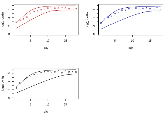
Figure 2.1: Observed values and the posterior predictive intervals for the three colonies
logarithm of growth, denoted by µ(t), changes over time according to the ODE dµ(t)
dt =θ1−θ2exp{µ(t)}, µ(0) = log(2),
as suggested in Ghosh and Goyal (2010). The three colonies are analyzed separately. In this example there are n = 18 observations for each colony. We put an inverse gamma prior on σ2 with shape and scale parameters 10 and 1 respectively and use w(t) = t7(1−t)7. Conditional onσ2we put Gaussian prior onβwith mean vector0and dispersion matrix nc−1k−1n σ2(XnTXn)−1 with c= 1000. We take m = 5 andkn = 2. The ODE has
the solution
µ(t) = logθ1+ log 2 +tθ1−log[2θ2(exp{tθ1} −1) +θ1].
2.7
Proofs of theorems
Proof of Theorem 2.1. The structure of the proof follows that of Proposition 3.1 of Brunel (2008) and Proposition 3.3 of Gugushvili and Klaassen (2012), but differs substantially in detail since we address posterior variation and also allow misspecification. First note that
Γ(f)−Γ(f0) =
Z 1 0
−(D0,0,1F(t, f0(t),θ0))TD0,1,0F(t, f0(t),θ0)w(t) (2.18) −d
dt[(D0,0,1F(t, f0(t),θ0))
Tw(t)] + (D
0,1,0S(t, f0(t),θ0))w(t)
(f(t)−f0(t))dt.
Interchanging the orders of differentiation and integration and using the definitions ofθ
and θ0,
Z 1
0
(D0,0,1F(t, f(t),θ))
T
(f0(t)−F(t, f(t),θ))w(t)dt = 0, (2.19)
Z 1
0
(D0,0,1F(t, f0(t),θ0))T (f00(t)−F(t, f0(t),θ0))w(t)dt = 0. (2.20)
Taking difference, we get
Z 1
0
(D0,0,1F(t, f(t),θ)−D0,0,1F(t, f(t),θ0))T(f00(t)−F(t, f0(t),θ0))
w(t)dt
+
Z 1 0
(D0,0,1F(t, f(t),θ0)−D0,0,1F(t, f0(t),θ0))T(f00(t)−F(t, f0(t),θ0))w(t)dt
+
Z 1
0
(D0,0,1F(t, f(t),θ0))T(f0(t)−f00(t) +F(t, f0(t),θ0)−F(t, f(t),θ0))w(t)dt +
Z 1 0
(D0,0,1F(t, f(t),θ)−D0,0,1F(t, f(t),θ0))T (f0(t)−f00(t) +F(t, f0(t),θ0)−F(t, f(t),θ0))w(t)dt
+
Z 1
0
Replacing the difference between the values of a function at two different values of an argument by the integral of the corresponding partial derivative, we get
M(f,θ)(θ−θ0) =
Z 1
0
(D0,0,1F(t, f(t),θ0)−D0,0,1F(t, f0(t),θ0))
T
(f00(t)−F(t, f0(t),θ0))w(t)dt
+
Z 1
0
(D0,0,1F(t, f(t),θ0))T (f0(t)−f00(t) +F(t, f0(t),θ0)−F(t, f(t),θ0))w(t)dt,
where M(f,θ) is given by
Z 1
0
(D0,0,1F(t, f(t),θ))T
Z 1
0
D0,0,1F(t, f(t),θ0+λ(θ−θ0))dλ
w(t)dt
−
Z 1
0
Z 1
0
(D0,0,1S(t, f(t),θ0+λ(θ−θ0)))dλ
w(t)dt
−
Z 1
0
Z 1
0
(D0,0,2F(t, f(t),θ0+λ(θ−θ0)))dλ
(f0(t)−f00(t) +F(t, f0(t),θ0)−F(t, f(t),θ0))w(t)dt.
Note thatM(f0,θ0) =J(θ0). We also define En ={(f,θ) : sup
t∈[0,1]
|f(t)−f0(t)| ≤n,kθ−θ0k ≤n},
wheren→0. By Lemmas 2.12 and 2.13, there exists a sequence{n}so that Π(Enc|Y) =
oP0(1). Then, M(f,θ) is invertible and the eigenvalues of [M(f,θ)]
−1 are bounded away from zero and infinity for sufficiently large n and
(M(f,θ))−1−(J(θ0)) −1
=o(1)
for (f,θ)∈En. Hence, uniformly on En
√
n(θ−θ0) = (J(θ0)) −1
for sufficiently large n, where
T1n =
Z 1
0
(D0,0,1F(t, f(t),θ0)−D0,0,1F(t, f0(t),θ0))
T
(f00(t)−F(t, f0(t),θ0))w(t)dt,
T2n =
Z 1
0
(D0,0,1F(t, f(t),θ0))T (f0(t)−f00(t))w(t)dt,
T3n =
Z 1
0
(D0,0,1F(t, f(t),θ0))
T
(F(t, f0(t),θ0)−F(t, f(t),θ0))w(t)dt.
In view of Lemmas 2.12 and 2.14, on a set in the sample space with high true probability, the posterior distribution of (J(θ0))
−1√
n(T1n+T2n+T3n) assigns most of its mass inside
a large compact set. Thus, we can assert that inside the set En, the asymptotic behavior
of the posterior distribution of √n(θ−θ0) is given by that of (J(θ0))
−1√
n(T1n+T2n+T3n). (2.21)
We shall extract √n(J(θ0)) −1
(Γ(f)−Γ(f0)) from (2.21) and show that the remainder term goes to zero. First write
T2n = −
Z 1
0
d
dt[(D0,0,1F(t, f0(t),θ0))
T
w(t)]
(f(t)−f0(t))dt
+
Z 1 0
(D0,0,1F(t, f(t),θ0)−D0,0,1F(t, f0(t),θ0))T (f0(t)−f00(t))w(t)dt,
which follows by integration by parts and the fact that w(0) = w(1) = 0. Note that the first integral of the above equation appears in (2.18). The norm of the second integral can be bounded above by a constant multiple of supt∈[0,1]|f(t)−f0(t)|2+supt∈[0,1]|f
0(t)−f0 0(t)|2 using the continuity of D0,1,1F(t, y,θ). Now we consider T3n in (2.21). Then,
T3n =
Z 1
0
(D0,0,1F(t, f0(t),θ0))T (F(t, f0(t),θ0)−F(t, f(t),θ0))w(t)dt
+
Z 1
0
(D0,0,1F(t, f(t),θ0)−D0,0,1F(t, f0(t),θ0))
T
The first integral on the right hand side of (2.22) can be written as
−
Z 1
0
(D0,0,1F(t, f0(t),θ0))
T
D0,1,0F(t, f0(t),θ0)(f(t)−f0(t))w(t)dt −
Z 1
0
(D0,0,1F(t, f0(t),θ0))T ×
Z 1
0
[D0,1,0F(t, f0(t) +λ(f−f0)(t),θ0)−D0,1,0F(t, f0(t),θ0)]dλ
×(f(t)−f0(t))w(t)dt = T31n+T32n,
say. Now T31n appears in (2.18). By the continuity of D0,2,0F(t, y,θ), kT32nk can be
bounded above up to a constant by a multiple of supt∈[0,1]|f(t)−f0(t)|2. We apply the Cauchy-Schwarz inequality and the continuity of D0,1,1F(t, y,θ) to bound the second
integral on the right hand side of (2.22) by a constant multiple of sup{|f(t)−f0(t)|2 : t∈[0,1]}. As far as the first term inside the bracket of (2.21) is concerned, we have
T1n =
Z 1
0
(D0,1,0S(t, f0(t),θ0)) (f(t)−f0(t))w(t)dt
+
Z 1
0
Z 1
0
(D0,1,0S(t, f0(t) +λ(f −f0)(t),θ0)−D0,1,0S(t, f0(t),θ0))dλ
×(f(t)−f0(t))w(t)dt.
The first integral appears in (2.18). The norm of the second integral of the above display can be bounded by a constant multiple of sup{|f(t)−f0(t)|2 : t ∈ [0,1]} utilizing the continuity ofD0,2,1F(t, y,θ) with respect to its arguments. Combining these, we find that the norm of the vector (J(θ0))
−1√
n(T1n+T2n+T3n)−(J(θ0)) −1√
n(Γ(f)−Γ(f0)) is bounded above by a constant multiple of
√ n sup
t∈[0,1]
|f(t)−f0(t)|2+ √
n sup
t∈[0,1]
|f0(t)−f00(t)|2.
Proof of Theorem 2.6. By Theorem 2.1 and (2.10), it suffices to show that
Π √n
d
X
j=1
GTn,jβj −
√
n(J(θ0)) −1
Γ(f0)∈ ·|Y
!
−N(µn, σ2Σn)
T V
=oP0(1). (2.23) Note that the posterior distribution ofGT
n,jβj is a normal distribution with mean vector
given by (1 +σ2ck
n/n)−1GTn,j(XnTXn)−1XnTY,j and dispersion matrix
σ2(1 +σ2ckn/n)−1GTn,j(X T
nXn)−1Gn,j.
We calculate the Kullback-Leibler divergence between two Gaussian distributions to prove the assertion. Alternatively, we can also follow the approach given in Theorem 1 and Corollary 1 of Bontemps (2011). The Kulback-Leibler divergence between the distribu-tions Np(µ1,Ω1) and Np(µ2,Ω2) is given by
1 2 tr(Ω
−1
1 Ω2) + (µ1−µ2)TΩ−11 (µ1−µ2)−p−log(det(Ω−11 Ω2))
.
Taking
µ1 = (1 +σ2ckn/n)−1GTn,j(X T
nXn)−1XnTY,j, Ω1 =σ2(1 +σ2ckn/n)−1GTn,j(X T
nXn)−1Gn,j
and µ2 =GTn,j(XnTXn)−1XnTY,j,Ω2 =σ2GTn,j(XnTXn)−1Gn,j, we get
tr(Ω−11 Ω2) =p+o(1). Also,
log(det(Ω−11 Ω2)) = plog(1 +σ2ckn/n)kn/n=o(1).
From the proof of Lemma 2.14, it follows that
(µ1 −µ2)TΩ1−1(µ1−µ2) n k2
n
n2Y
T
,j Xn(XnTXn)−1Gn,jGTn,j(X T
nXn)−1XnTY,j
. nk 2
Hence, the total variation distance between the posterior distribution of GT
n,jβj and a
Gaussian distribution with mean GT
n,j(XnTXn)−1XnTY,j and dispersion matrix given by
σ2GT
n,j(XnTXn)−1Gn,j converges in P0-probability to zero for j = 1, . . . , d. Since the posterior distributions of βj and βj0 are mutually independent forj 6=j0; j, j0 = 1, . . . , d,
we can assert that the posterior distribution of √nPd
j=1G
T n,jβj −
√
n(J(θ0)) −1
Γ(f0) can be approximated in total variation by N(µn, σ2Σn).
Proof of Theorem 2.7. The marginal posterior of σ2 is also inverse gamma with pa-rameters (dn+ 2a)/2 and b +Pd
j=1Y
T
,j(In−PXn(1 + (ckn/n)) −1)Y
,j/2, where PXn =
Xn(XnTXn)−1XnT. Straightforward calculations show that
E(σ2|Y) = 1 2 Pd j=1 YT
,jY,j−Y,jTPXnY,j(1 +cknn
−1)−1 +b 1
2dn+a−1
,
Var(σ2|Y) = (E(σ 2|Y))2 1
2dn+a−2 ,
which give rise to|E(σ2|Y)−σ2
0|=OP0(n
−1/2) and Var(σ2|Y) = O
P0(n
−1). In particular, the marginal posterior distribution of σ2 is consistent at the true value of error variance. LetN be an arbitrary neighborhood of σ0. Then, Π(N c|Y) =oP0(1). We observe that
sup
B∈Rp
Π(
√
n(θ−θ0)∈B|Y)−Φ(B;µn, σ02Σn)
≤
Z
sup
B∈Rp
Π(
√
n(θ−θ0)∈B|Y, σ)−Φ(B;µn, σ2Σn)dΠ(σ|Y)
+
Z
sup
B∈Rp
Φ(B;µn, σ2Σn)−Φ(B;µn, σ02Σn)
dΠ(σ|Y)
≤ sup
σ∈N sup
B∈Rp
Π(
√
n(θ−θ0)∈B|Y, σ)−Φ(B;µn, σ2Σn)
+ sup
σ∈N,B∈Rp
Φ(B;µn, σ2Σn)−Φ(B;µn, σ02Σn)
+ 2Π(N c|Y).
consistency. Hence, we get the desired result.
Proof of Theorem 2.8. According to the fitted model, Yi,1×d ∼ Nd((Xn)i,Bn,Σd×d) for
i= 1, . . . , n. The logarithm of the posterior probability density function (p.d.f.) is nega-tive half times
n
X
i=1
((Xn)i,Bn−Yi,)Σ−1 BnT(X T
n),i−Yi,T
+
d
X
j=1
βjT X T nXn
nc−1k−1
n
βj, (2.24)
where Bn = (β1, . . . ,βd). The quadratic term in βj above for j = 1, . . . , d, can be consolidated to
tr
Σ−1+cknId n
BnTXnTXnBn
. (2.25)
The term in (2.24) which is linear inβj, j = 1, . . . , d, is given by n
X
i=1
(Xn)i,(β1. . .βd)Σ−1Yi,T = tr XnBnΣ−1YT
= tr Σ−1YTXnBn
.
A completing square argument shows that the posterior density is proportional to
exp −1 2tr
Σ−1 +cknId n
Bn−(XnTXn)−1XnTYΣ
−1
Σ−1+ cknId n
−1!T
XnTXn Bn−(XnTXn)−1XnTYΣ
−1
Σ−1+cknId n
−1!#)
,
which can be identified with the pdf of a matrix normal distribution. More precisely,
vec(Bn)|Y ∼ N vec (XnTXn)−1XnTYΣ−1
Σ−1+ cknId n
−1!
,
Σ−1 +cknId n
−1
⊗(XnTXn)−1
!
.
Fixing a j ∈ {1, . . . , d}, we observe that the posterior mean of βj is a weighted sum of
order of 1, whereas for j0 6=j, the contribution from (XT
nXn)−1XnTY,j0 is of the order of
kn/n which goes to zero as n goes to infinity. Thus, the results of Lemmas 2.11 to 2.14
can be shown to hold under this setup. We are interested in the limiting distribution of (J(θ0))
−1
Γ(f) = Pd
j=1G
T
n,jβj = (GTn,1. . .GTn,d)vec(Bn). We note that the posterior
distribution of (Σ−1+cknId/n)
1/2
⊗Ikn+m−1
vec(Bn) is a (kn+m−1)d-dimensional
normal distribution with mean vector and dispersion matrix being given by vec(XnTXn)−1XnTYΣ
−1 Σ−1+ck
nId/n
−1/2
and Id⊗(XnTXn)−1 respectively, since by the properties of Kronecker product, for the matrices A, B and D of appropriate orders (BT ⊗A)vec(D) = vec(ADB).
Let us consider the mean vector of the posterior distribution of the vector
Σ−1 +cknId/n1/2⊗Ikn+m−1
vec(Bn). We observe that
(XnTXn)−1XnTYΣ
−1
Σ−1+cknId n
−1/2
= (XnTXn)−1XnT(Y,1. . .Y,d)
Σ+cknΣ 2 n
−1/2
= (XnTXn)−1XnT d
X
j=1
Y,jcj1. . .
d
X
j=1
Y,jcjd
!
,
where Cn = ((cjk)) = (Σ+kncΣ2/n)
−1/2
. For k = 1, . . . , d, we define Zk to be the
sub-vector consisting of [(k−1)(kn+m−1) + 1]th to [k(kn+m−1)]th elements of the vector
given by
Σ−1+cknId
n
1/2
⊗Ikn+m−1
vec(Bn). Then we have
Zk|Y ∼Nkn+m−1 (XnTXn)
−1
XnT d
X
j=1
Y,jcjk,(XnTXn)
−1
!
.
Also, the posterior distributions ofZkandZk0are mutually independent fork 6=k0;k, k0 =
distribu-tion of Zk and N
(XnTXn)
−1
XnT Pd
j=1Y,jσjk,(XnTXn)
−1
converges in P0-probability to zero for k = 1, . . . , d, where Σ−1/2 = ((σjk)). The total variation distance between two
multivariate normal distributions with equal dispersion matrix (XT
nXn)−1and mean
vec-tors (XT nXn)
−1
XT n
Pd
j=1Y,jcjk and (X
T nXn)
−1
XT n
Pd
j=1Y,jσ
jk is bounded by the
quan-tity Pd
j=1
(X
T nXn)
−1/2
XT
nY,j(cjk−σjk)
. Fixing k, for j = 1, . . . , d, we have that
(X
T nXn)
−1/2
XnTY,j(cjk−σjk)
= |cjk−σ
jk|YT
,jXn(XnTXn)
−1
XnTY,j
1/2
≤ |cjk−σjk| Y,jTY,j
,
since the eigenvalues ofXn(XnTXn)−1XnT are either zero or 1. Since clearlyCnconverges toΣ−1/2 at the ratekn/n, we have for j = 1, . . . , d,
(X
T nXn)
−1
XnTY,j(cjk −σjk)
.
kn
n OP0( √
n) =oP0(1). (2.26) Hence, we conclude that the total variation distance between the distributions
N (XnTXn)
−1
XnT d
X
j=1
Y,jcjk,(XnTXn)
−1
!
and N(XT nXn)
−1
XT n
Pd
j=1Y,jσ
jk,(XT nXn)
−1
converges to zero in P0-probability. We can write GT
n,1. . .GTn,d
vec(Bn) in terms of Zk as d
X
k=1
colsk(k(k−1)(n+mkn+−1)m−1)+1
GTn,1. . .GTn,d
Σ−1+ cknId n
1/2
⊗Ikn+m−1
!−1 Zk.
Since the posterior distributions ofZk,k= 1, . . . , d, are independent, we therefore obtain
that
√
n GTn,1. . .GTn,d
vec(Bn)−
√
n(J(θ0)) −1
(f0)
−N(µ∗∗n ,Σ∗∗n)
where µ∗∗n is given by
√ n
d
X
k=1
colsk(k(k−1)(n+mkn+−1)m−1)+1
GTn,1. . .GTn,d
Σ−1+cknId n
1/2
⊗Ikn+m−1
!−1
×(XnTXn)
−1
XnT d
X
j=1
Y,jσjk −(J(θ0)) −1√
nΓ(f0),
and Σ∗∗n is given by
n
d
X
k=1
colsk(k(k−1)(n+mkn+−1)m−1)+1
GTn,1. . .GTn,d
Σ−1+cknId n
1/2
⊗Ikn+m−1
!−1
×(XnTXn)
−1
×rowsk(k(k−1)(n+mkn+−1)m−1)+1
Σ−1+cknId n
1/2
⊗Ikn+m−1
!−1
GTn,1. . .GTn,dT
.
Following the steps of the proof of Lemma 2.14, it can be shown that the eigenvalues of the matrix Σ∗n mentioned in the statement of Theorem 2.8 are bounded away from zero and infinity. We can show that the Kullback-Leibler divergence ofN(µ∗∗n,Σ∗∗n) from N(µ∗n, σ2Σ∗n) converges in probability to zero by going through some routine matrix manipulations. Hence,
√
n GTn,1. . .GTn,dvec(Bn)−√n(J(θ0))−1(f0)−N(µ∗n, σ2Σ∗n)
T V =oP0(1). The above expression is equivalent to (2.23) of the proof of Theorem 2.6. Following steps similar to those of Theorem 2.6, we get (2.13). We obtain (2.14) by following the proof of Theorem 2.7.
Proof of Remark 2.10. Using the definition (2.17) we get
Z 1
0
(D0,0,0,1F1(t, f1(t), f2(t),θ))T (f10(t)−F1(t, f1(t), f2(t),θ))w(t)dt = 0,
Z 1 0
(D0,0,0,1F1(t, f1θ0(t), f2θ0(t),θ0))
T
Subtracting the latter from the former we get
Z 1
0
(D0,0,0,1F1(t, f1(t), f2(t),θ))
T
(f10(t)−F1(t, f1(t), f2(t),θ))w(t)dt −
Z 1 0
(D0,0,0,1F1(t, f1(t), f2θ0(t),θ))
T
(f10(t)−F1(t, f1(t), f2θ0(t),θ))w(t)dt
+
Z 1
0
(D0,0,0,1F1(t, f1(t), f2θ0(t),θ))
T
(f10(t)−F1(t, f1(t), f2θ0(t),θ))w(t)dt −
Z 1
0
(D0,0,0,1F1(t, f1θ0(t), f2θ0(t),θ0))
T
(f10θ0(t)−F1(t, f1θ0(t), f2θ0(t),θ0))w(t)dt
=0.
Since f2θ0(t) is a known function of t, it can be absorbed in the first argument of F1 which then becomes a function of three arguments. Then the second part of the left side above can be analyzed as in Theorem 2.1. To deal with the first part of left side it is sufficient to study the differencef2(·)−f2θ0(·). Note that f2(t) can be written as
φn(t, f1θ0(t),θ0) + (f1(t)−f1θ0(t))D0,1,0φn(t, f1θ0(t),θ0) +(θ−θ0)TD0,0,1φn(t, f1θ0(t),θ0) +O (f1(t)−f1θ0(t))
2
+O kθ−θ0k2
.
Also, the difference supt∈[0,1]|φn(t, f1θ0(t),θ0)−f2θ0(t)| is of the order n
−1. Now using Lemmas 2.11 to 2.13, we can conclude that
k√n(θ−θ0)−Jθ−10 √n(Γ(f1)−Γ(f1θ0))k →0
as n→ ∞. Now we can prove the Bernstein-von Mises theorem as before.
2.8
Proofs of the lemmas
Lemma 2.11. For m ≥2 and kn satisfying n1/2m knn, for r = 0,1,
sup
t∈[0,1]
|E0(E(f(r)(t)|Y))−f (r)
0 (t)|=o(k
r+1/2
n /
√ n).
Proof. We note that f(r)(t) = (N(r)(t))Tβ for r= 0,1 with N(r)(·) standing for the rth order derivative of N(·). By (2.6),
E(f(r)(t)|Y) =
1 + cknσ 2 n
−1
(N(r)(t))T(XnTXn)
−1
XnTY. (2.27)
Theorem A.1 gives
(N(r)(t))T(XnTXn)
−1
N(r)(t) k 2r+1
n
n . (2.28)
Since f0(r) ∈ C(m−r), there exists a β∗ (De Boor, 1978, Theorem XII.4, page 178) such that
sup
t∈[0,1]
|f0(r)(t)−(N(r)(t))Tβ∗|=O(kn−(m−r)). (2.29)
For any t ∈ [0,1], we can bound the absolute bias of E(f0(r)(t)|Y) multiplied with √
nk−nr−1/2 by
√
nk−nr−1/2 sup
t∈[0,1]
|E0(E(f(r)(t)|Y))−f (r) 0 (t)| ≤ √nk−nr−1/2 sup
t∈[0,1]
1 + cknσ 2 n
−1
(N(r)(t))Tβ∗−(N(r)(t))Tβ∗
+√nkn−r−1/2
1 + cknσ 2 n
−1
sup
t∈[0,1]
|(N(r)(t))T(XnTXn)
−1
XnT(f0(x)−Xnβ∗)|
+√nkn−r−1/2 sup
t∈[0,1]
|f0(r)(t)−(N(r)(t))Tβ∗|.
Using the fact that supt∈[0,1]|(N(r)(t))Tβ∗| = O(1), first term on the right hand side of the previous inequality is of the order of k−nr+1/2/
√
√ nk−m
n . The third term has the order of
√
nk−nm−1/2 as a result of (2.29). By the assumed
conditions onm and kn, the assertion holds.
The following lemma controls posterior variability.
Lemma 2.12. If m≥5 and n1/2m k
nn1/8, then for r= 0,1 and for all >0,
Π √n sup
t∈[0,1]
|f(r)(t)−f(r) 0 (t)|
2 > |Y
!
=oP0(1).
Proof. By Markov’s inequality and the fact that |a+b|2 ≤ 2(|a|2 +|b|2) for two real numbers a and b, we can bound Πsupt∈[0,1]√n|f(r)(t)−f(r)
0 (t)|2 > |Y
by 2 √ n ( sup
t∈[0,1]
E(f
(r)(t)|Y)−f(r) 0 (t) 2 + E " sup
t∈[0,1]
f(r)(t)−E(f(r)(t)|Y) 2 |Y #) .(2.30)
Now we obtain the asymptotic orders of the expectations of the two terms inside the bracket above. We can bound the expectation of the first term by
2 sup
t∈[0,1]
E0(E(f
(r)(t)|Y))−f(r) 0 (t) 2 +2E0 " sup
t∈[0,1]
E(f(r)(t)|Y)−E0(E[f(r)(t)|Y])
2
#
. (2.31)
Using (2.27), supt∈[0,1]
E(f(r)(t)|Y)−E0(E[f(r)(t)|Y])
can be bounded up to a constant
multiple by
max 1≤k≤n
(N
(r)
(sk))T(XnTXn)
−1
XnTε
+ sup
t,t0:|t−t0|≤n−1
(N
(r)(t)−N(r)(t0
))T(XnTXn)
−1
XnTε
,
where sk =k/n for k = 1, . . . , n. Applying the mean value theorem to the second term
term of (2.31) by a constant multiple of
max 1≤k≤n
(N
(r)(s
k))T(XnTXn)
−1
XnTε
2
+ sup
t∈[0,1] 1 n2
(N
(r+1)(t))T(XT nXn)
−1
XnTε
2
.(2.32)
By the spectral decomposition, we can write Xn(XnTXn)−1XnT = PTDP, where P is an orthogonal matrix andD is a diagonal matrix withkn+m−1 ones andn−kn−m+ 1
zeros in the diagonal. Now using the Cauchy-Schwarz inequality, we get
E0
max 1≤k≤n
(N
(r)
(sk))T(XnTXn)
−1
XnTε
2
≤ max 1≤k≤n
n
(N(r)(sk))T(XnTXn)
−1
N(r)(sk)
o
E0 εTPTDP ε
.
By Theorem A.1 and the fact that Var0(P ε) = Var0(ε), we can conclude that the expectation of the first term of (2.32) isO(k2r+2
n /n). Again applying the Cauchy-Schwarz
inequality, the second term of (2.32) is bounded by
sup
t∈[0,1]
1 n2(N
(r+1)
(t))T(XnTXn)−1N(r+1)(t)
(εTε),
whose expectation is of the order n(kn2r+3/n3) = k2nr+3/n2, using Theorem A.1. Thus, the expectation of the bound given by (2.32) is of the order k2nr+2/n. Combining it with (2.31) and Lemma 2.11, we get
E0
"
sup
t∈[0,1]
E(f
(r)(t)|Y)−f(r) 0 (t) 2# =O
k2r+2
n
n
. (2.33)
Define
ε∗ := (XnTXn)1/2β−
1 + σ 2ck
n
n
−1
(XnTXn)−1/2XnTY. Note that
ε∗|Y ∼N(0, σ−2+ckn/n
−1
Ikn+m−1).
Expressing supt∈[0,1]|f(r)(t)−E[f(r)(t)|Y]|as sup
t∈[0,1]
(N
(r)(t))T(XT nXn)
−1/2
ε∗
us-ing the Cauchy-Schwarz inequality and Theorem A.1, the second term inside the bracket in (2.30) is seen to be O(k2r+2
n /n). Combining it with (2.30) and (2.33) and using
2r+ 2 ≤4, we have the desired assertion.
Lemmas 2.11 and 2.12 can be used to prove the posterior consistency of θ as shown in the next lemma.
Lemma 2.13. If m ≥ 5 and n1/2m k
n n1/8, then for all > 0, Π(kθ−θ0k > |Y) =oP0(1).
Proof. By the triangle inequality, using the definition in (2.7), |Rf(η)−Rf0(η)| ≤ kf
0(·)−
f00(·)kw +kF(·, f(·),η)−F(·, f0(·),η)kw
≤ c1 sup
t∈[0,1]
|f0(t)−f00(t)|+c2 sup
t∈[0,1]
|f(t)−f0(t)|,
for appropriately chosen constantsc1 andc2. We denote the setTn={f : supt∈[0,1]|f(t)− f0(t)| ≤ τn, supt∈[0,1]|f
0
(t)−f00(t)| ≤ τn} for some τn →0. By Lemma 2.12, there exists
such a sequence {τn} so that Π(Tnc|Y) = oP0(1). Hence for f ∈Tn,
sup
η∈Θ
|Rf(η)−Rf0(η)| ≤(c1+c2)τn=o(1)
Therefore, for any δ > 0, Π(supη∈Θ|Rf(η)−Rf0(η)| > δ|Y) = oP0(1). By assumption (2.8), for kθ−θ0k ≥ there exists a δ >0 such that
δ < Rf0(θ)−Rf0(θ0) ≤ Rf0(θ)−Rf(θ) +Rf(θ0)−Rf0(θ0) ≤ 2 sup
η∈Θ
|Rf(η)−Rf0(η)|,
since Rf(θ)≤Rf(θ0). Consequently,
Π(kθ−θ0k> |Y)≤Π
sup
η∈Θ
|Rf(η)−Rf0(η)|> δ/2|Y
The asymptotic behavior of the posterior distribution of√n(J(θ0)) −1
(Γ(f)−Γ(f0)) is given by the next lemma.
Lemma 2.14. Under the conditions of Theorem 2.6, on a set in the sample space with
high true probability, the posterior distribution of √n(J(θ0)) −1
(Γ(f)−Γ(f0)) assigns
most of its mass inside a large compact set.
Proof. First note that
(J(θ0)) −1
Γ(f) =
d
X
j=1
GTn,jβj
and (J(θ0)) −1
Γ(f0) =
Pd
j=1
R1
0 A,j(t)fj0(t)dt, whereA,j(t) denotes thej
thcolumn of the
matrixA(t) as defined in Remark 2.5 forj = 1, . . . , d. In order to prove the assertion, we will show that Var(GTn,jβj|Y) andVar0(E(GTn,jβj|Y)) have all eigenvalues of the order n−1 and
max 1≤k≤p
[E0(E(GTn,jβj|Y))]k−
Z 1
0
Ak,j(t)fj0(t)dt
= o n−1/2,
fork = 1, . . . , p,j = 1, . . . , d, whereAk,j(t) is the (k, j)th element of the matrixA(t). Let
us fixj ∈ {1, . . . , d}. We note that
E(GTn,jβj|Y) =
1 + cknσ 2 n
−1
GTn,j(XnTXn)−1XnTY,j.
Hence,
Var0(E(GTn,jβj|Y)) = σ20
1 + σ 2ck
n
n
−2
GTn,j(XnTXn)
−1
Gn,j.
Also note that
Var(GTn,jβj|Y) = σ2
1 + σ 2ck
n
n
−1
GTn,j(XnTXn)−1Gn,j.
If Ak,j(·) ∈ Cm
∗
and αT
k,j = (Ak,j(t∗1), . . . , Ak,j(t∗kn+m−1)) with appropriately chosen t∗1, . . . , t ∗
kn+m−1. We can express GT
n,j(XnTXn)−1Gn,j as
(Gn,j−G˜n,j)T(XnTXn)−1(Gn,j −G˜n,j) + ˜GTn,j(X T
nXn)−1(Gn,j−G˜n,j)
+ ˜GTn,j(XnTXn)−1Gn,j˜ + (Gn,j −Gn,j˜ )T(XnTXn)−1Gn,j˜
where [ ˜GTn,j]k, =
R1
0 A˜k,j(t)(N(t))
Tdt for k = 1, . . . , p. Let ˜A = (( ˜A
k,j)). We study the
asymptotic orders of the eigenvalues of the matrices ˜GTn,j(XnTXn)−1Gn,j˜ and (Gn,j − ˜
Gn,j)T(XnTXn)−1(Gn,j−G˜n,j). Note that
αTk,j
Z 1
0
N(t)NT(t)dtαk,j =
Z 1
0 ˜
A2k,j(t)dt kαk,jk2k−1n ,
by Theorem A.1 implying that the eigenvalues of the matrix R01N(t)(N(t))Tdt are of
orderkn−1. The eigenvalues of XnTXn/n
are of the order kn−1 by Theorem A.1. Then we have
maxeigG˜Tn,j(XnTXn)−1G˜n,j
. kn
nmaxeig
˜
GTn,jG˜n,j
= kn
nmaxeig
Z 1
0 ˜
A,j(t)NT(t)dt
Z 1
0
N(t)( ˜A,j(t))Tdt
= kn
nmaxeig (α1,j· · ·αp,j)
T Z 1
0
N(t)NT(t)dt
2
(α1,j· · ·αp,j)
!
. 1
nkn
maxeig((αTk,jαl,j))
1
nmaxeig((hAk,j(·), Al,j(·)i))
= 1
nmaxeig (Bj) 1 n.
Similarly, it can be shown that mineig
˜
GTn,j(XnTXn)−1Gn,j˜