Development of an Imputation Technique –
INI for Software Metric Database with
Incomplete Data
Rashidah F. Olanrewaju1 Wasito Ito 1
Dept. of Electrical and Computer Engineering, Kulliyyah of Engineering, International Islamic University, Jalan Gombak, 50728 Kuala Lumpur, Malaysia (Email: [email protected])
Abstract - Software metrics are numerical data that provides a quantitative basis for the development and validation of models, and effective measurement of the software development process. Gathering software engineering data can be expensive. Such precious and costly data cannot afford to be missing. However missing data is a common problem and software engineering database is not an exception. Though there are many algorithms to solve problem of incomplete data, unfortunately few have been developed in the field of Software Engineering. Missing data causes significant problem. With inaccurate data or missing data, it is very difficult to know how much a project will cost or worth. Missing data leads to loss of information, causes biasness in data analysis and hence results to inaccurate decision-making for project management and implementation.
In this paper, an imputation technique for imputing missing data based on global–local Modified Singular Value Decomposition (MSVD) algorithm, INI was proposed. This technique was used for estimating missing data in a software engineering database (PROMISE). Its performance was evaluated and compared with two existing imputation techniques, Expectation Maximization (EM) and Mean Imputation (MI). Varying percentages of missings, (1%, 10%, 15%, and 20% 25%) were introduced in the original dataset in order to have an incomplete dataset for imputation. Simulations were carried for comparative purposes.
Imputation Error (IE) was use as an evaluation criterion. Study results showed that, the only method that consistently outperformed other methods (EM and MI), guarantee a higher accuracy of imputed data, prompt and less bias at all level of missings is the global-local MSVD, INI. It maintained consistency at all level of missings compared to EM and MI. It was found that EM is not suitable for data with missing proportion greater than 20%. While MI lost in all count to EM and INI.
Index terms – data imputation, missing data, software engineering database, k-NN, MSVD based imputation.
I. INTRODUCTION
The meticulous effort put in collecting software engineering data is to make sure that the collected data can provide useful information for project, process, and quality management and, at the same time, that the data collection process will not be a burden on development teams. Therefore, it is important to handle the data collected carefully and properly. Gathering software engineering data can be expensive, especially if it is done as part of a research program. For example, Kan [2] reported that the NASA
Software Engineering Laboratory spent about 15% of their development costs on gathering and processing data on hundreds of metrics for a number of projects.
It was found that missing data are often encountered in software engineering database that are used to construct effort predictive models, software cost estimation models etc [3],[6],[7]. The fact is that most of the software databases suffer from this missingness problem. Even the databases from International Software Benchmarking Standard Group (ISBSG) database have more than 40% of their variables incomplete [3]. It was reported in [9] that missing data in software engineering may substantially affect data analysis. This problem makes it difficult to develop the software cost estimation models, effort predictive models etc.
Little & Rubin [5] discovered that the problem of handling missing data has been treated adequately in various real world data sets. Several statistical methods have been developed since the early 1970s. However little has been done within the context of software engineering data analysis [10]. Missing data causes significant problems in data analysis of software metric data. This is because decision-making often relies on relevant information extracted from such data. Lack of complete/missing data in several important projects is a common phenomenon, which may cause misleading results regarding the models accuracy and prediction ability.
There are several reasons why observations may have missing values. Within the domain of software engineering, lack of time, cost of gathering data, lack of commitment, lack of training and political reasons (refusal to release figures that “look bad”)[7].
With inaccurate data or missing data, it is very difficult to know how much a project will cost or will worth. It also causes improper project management and inefficient time management to complete the project. Missing values will lead to loss of information and biasness in data analysis and hence results to inaccurate decision.
There are basically three ways to handle incomplete data or missing values known as Missing Data Techniques (MDTs) [3]. They can be categorized according to the approach each is used for. The most popular is to discard unit whose information is incomplete by Case Deletion, also known as Listwise Deletion (LD). Another option is to fill the vacuity with some Imputation techniques such as Mean Imputation (MI), Similar Response Pattern Imputation
(SRPI), Hot Deck Imputation, and Regression Imputation, etc. Imputation-based method is to replace missing values with the suitable estimated values. Which is a better solution that does not require removal of useful information, hence increasing the amount of data usability as suggested in [9]. Other alternative is to use a Model-Based method that can analyse incomplete dataset directly such as Full Information Maximum Likelihood (FIML), Expectation Maximization (EM) etc [3]. In this study, an imputation technique, Global-local Modified Singular Value Decomposition (MSVD) based algorithm, INI is proposed, which has inbuilt combination features of both k-NN and the computational properties of SVD, that makes it a powerful tool for data imputation. INI will give more accurate values of the missings, because SVD find the best singular value and put in the missing entries. This combined method would treat the problem of imputation as a machine-learning problem.
II. OBJECTIVE OF STUDY
The objectives of this study are:
To analyze the performance of the MSVD algorithm as an imputation technique for completing software metrics dataset in software engineering database. The completed database can thereby be used for software engineering models like software cost estimation models, effort predictive models etc.
To compare the proposed technique, MSVD algorithm as an imputation method with the existing imputation techniques, such as Mean Imputation (MI), Expectation Maximization (EM), in order to evaluate each method’s accuracy.
III. RESEARCH METHOD
In this section, we described how MSVD works in relation with k-NN, and how its properties affect imputation. Also the strategies of neighbours’ selection are also discussed. Since INI is combination of MSVD and k-NN, therefore a brief explanation of each algorithm is explained
A. K-NN
In this method, the missing values of an instance are imputed considering a given number of instances that are most similar (closer) to the instance of interest. The similarity of the two instances is determined using a distance function. Euclidean distance squared was used, due to its compatibility with least square (minimal error). Any entity with one or more missing entries is considered as a target
entity to be imputed. The distance between target entity Ai
and an entity Ajis defined as:
D2 (AiAj M) = [aik -ajk] 2 mik mjk; for i, j = 1,2,…N
Where mik and mjk are missing value for aik and ajk
respectively.
K-NN contains 3 main steps: 1. Search for the target entity
2. Find its k nearest neighbours based on metric distance (Euclidean), Numbers of neighbours will depend on the specification of k, for this study, k= 5 were chosen. The 5 neighbours are inclusive of the target entity. Only the rows with non-missing entries were considered as the target row’s neighbours.
3. Impute the missing entries at the target entity
B. Modified SVD
This method is generated from the weighted least square minimization problem. This approach consists of iteratively performing ordinary least squares minimization problem by adjusting the solutions found to majorise the function [4]. This method is called Iterative Majorization Least Squares (IMLS) .The algorithm starts with a completed data matrix Adenoted by Aswere s = 1,2… is number of iteration. At each iteration s,the algorithm finds the best factor of SVD decomposition of As and imputes the found result into the missing entries. This is updated before the next iteration starts. IMLS is the brain power of MSVD
C. Generation of missings structure.
Missings is an mxn matrix that consists of 0’s and 1’s denoted by M. “1” represents an observed data while “0” represents a missing data. Programs were written in Matlab programming language to generate a random uniform distribution for the missing proportion of 1%, 10%, 15% and 25%. The missings were stored in Serand
D. Simulation approach
An actual dataset with no missing was used from
PROMISE Software Engineering Repository, [1]
(SERepository) along with creation of missing pattern (1%, 10%, 15%, 20%, & 25%) on the said data. Afterwards, the three different Missing Data Techniques (MDTs) namely: INI, EM and MI were applied. Setting MI as the benchmark for comparison. Each of this point i.e. MDTs, percentage of missing data, number of instance and their permutations were all combined and simulated for 200times x 5patterns. Subsequently, computation of Imputation Error of each MDTs was carried out. Performances of each were evaluated and compared using their imputation error (differences between the original values and the imputed values).
D1. Steps involved in INI: Step 1: Creating missing data
The experiment was carried out by selecting randomly a data matrix A from SERepository(original data with no missings) and a corresponding missing matrix M
from the Serand of specified percentage of missing (1%, 10%, 15%, 20% and 25%). Matrix A and M are both of same size 50x15. Matrix A is used to multiply Min order to create missing structure in matrix A. The results were stored in A*.
Step 2: Imputations
IMLS was applied globally on matrix A* to impute all the data entries both missing and non missing (update). Thus A*, is a complete matrix. Subsequently, a target row
Ai, was selected and its neighbours based on the number of
specified neighbours, here, neighbour k =5. This was done using the k-NN version of imputation. As a result, a sub data matrix of 5 rows from matrix A* with a missing structure named matrix Akwas obtained.
A local version of IMLS was used on matrix Akto impute the value of Ai of A* which resulted in a complete
the only value that was transferred to matrix A* to replace the missings value. These processes continued until all the missing in matrix A* were all imputed. As a result, a complete matrix X with no missings was obtained.
Step 3:Evaluation of results
Since the original data contains no missing, and missings were generated separately from the selected data, evaluation of the quality of the imputation can be done by comparing the imputed value with the original data. A squared Imputation Error, IE was used to appraise the performance of the algorithm.
! !
! !
" " " "
# # #
"
N i
n
j ij ij
N i
n
j ij ij ij
a m
a a m
1 1
2
1 1
2 *
) 1 (
) )( 1 (
IE
(1)
Where mij is the missing matrix entry and aij is the data
matrix a* with imputed values.
VI. EXPERIMENTAL RESULTS AND DISCUSSION
Table 1 shows the results of 1000 experiments made up of 200 (50x15 size matrix) dataset with five missings patterns. The missing patterns are 1%, 10%, 15%, 20%, and 25%. The mean error was recorded in columns for different missing patterns with corresponding standard deviation.
Table 1
From Table 1, the obvious winner, at each level of missings, that is, 1% through 25% missings was the global-local MSVD method, INI, followed by EM then MI. The results of MI, for missing patterns from 1% through 20% were poor due to very high error. Although at 25%, there was a sudden improvement in its performance, which was even better than EM. On the other hand, it is pertinent to note that for EM, which was the second best, when the missing grows to 25%, it was observed that the error drastically and hugely increased and fell out of range.
A number of conclusions can be drawn from the table: The result got using MI (bench mark) reflects its poor performance when the percentage missingness is small. Therefore as the percentage of missings decreased, the performance measured decreased as well. It showed that MI lacks precision in the distribution since all the missing values are imputed at the centre of the distribution. Based on the result obtained using MI at 1% through 20%, it may not be suitable for imputing data with missing percentage below 20%. MI imputation is significantly better than EM as the missingness grows from 20% to 25%.
For EM, the largest error obtained was at 25%. There is more flux in the performance of EM, especially at higher percentage of missings. EM lost it credibility when
the missings become large, therefore it may not be suitable for data with large missings, precisely 25% missings. The reason for such instability and erratic behaviour of EM at 25% was observed during the computation of error of missing data imputation. There was a wide variation of imputation error values in EM. In a typical dataset at 25% of missings, there was as minimal value of imputation error as low as 0.008496, which soared to 1.13E+112. This has a cumulative effect on the mean error and standard deviation. With this kind of variation, there is tendency that the mean and standard deviation for such percentage of missings will be volatile and will create biasness in such data analysis. Consequently, analysis with such data will lack efficiency, which may lead to taking wrong decisions.
In contrast, INI showed a good data stability, which gave the best performances due to it low imputation error at all level of missings. INI is the overall winner with less variation in terms of error and higher precision in terms of performance. INI performance was the best at all level of missings compared to MI and EM. However, these conclusions may be blurred due to the outlier values especially in EM. Due to this observation, all outliers are removed and thus graphs in figure 3.1 to 3.5 are used for further analysis.
.
V. EFFECT OF MISSINGNESS IN RELATION WITH MEAN ERROR FOR VALUES WITHOUT OUTLIERS.
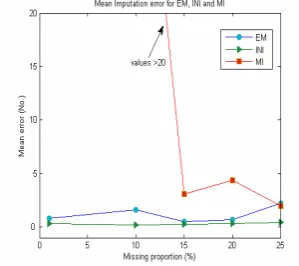
Figure 1.1 shows a typical plot of mean error for EM, INI with MI, as the bench mark. Against the missing proportions, in which 1, 10, 15, 20, 25 represent the percentage of missings. The mean error was obtained by computing Imputation Error for each percentage of missings (1%, 10%, 15%, 20%, and 25%). For each percentage of missings, there are 200 datasets. For each of the datasets, an imputation error was computed thus 200 sets of imputation errors were obtained for each percentage of missings. Finally the mean error was computed for each percentage of missings based on the imputation error obtained. Removing the outliers’ error especially for EM at 25% missings before computing the mean error plotted the graph drawn. Outliers are errors above 1000.
Figure 1.1: Levels of missing with the mean imputation error for the three techniques EM, INI and MI at 1%, 10%, 15%, 20%, 25% missings.
From Figure 1.1, it will be observed that for the bench mark, MI, as the percentage of missings increases from 1 to 10; the mean error decreases. This decrease continues till missings reached 15% where the mean error slightly increased. However from 20% missings, it gradually
decreased till the experiment was terminated. On the other hand, for EM, as the percentage of missings increased from 1% to 10%, the mean error increased slowly. However, from 10% to 15% missings, the mean error decreases. But from 15% to 20% there was a slight increase which shot up at 25% missing when the experiment was terminated. Finally for INI, as the percentage of missings increased from 1% to 10% the mean error decreased slightly, however, from 10% through 25% missings, INI maintains a consistent mean error increase when the experiment was terminated.
A. Imputation techniques performance compared pair- wise
Missing proportion of EM and MI are plotted against the mean error in Figure 1.2. The result showed that EM has better performance at 20% and below than MI. However its performance was inconsistent as the missings increased to 25%, it performance tends to decline which it measure almost same mean error with MI.. In contrast, performance of MI was best at 25%. This indicates that as the missingness increased to 25%, EM performance decline while MI tends to perform better and ability to compete with EM.
Figure 1.2: Levels of missings with the mean imputation error for EM and MI (bottom line) at 1%, 10%, 15%, 20%, 25% missings.
It can be seen from Figure 1.3 where INI and MI are compared. The mean error of INI was low compared to MI at all levels of missings, INI is more accurate than MI. It can be observed that at all levels of missings for INI, the lower the missing proportion, the higher the accuracy of the imputed data and the lesser the error obtained. This is a good indicator that INI is less likely to introduce bias in data analysis than MI. INI performance is consistent at all levels of missings. It is more robust and less bias than MI
Figure 1.3: Levels of missings with the mean imputation error for INI and MI at 1%, 10%, 15%, 20%, 25% missings.
From Figure 1.4, the comparison between EM and INI was carried out. It was found that performance of EM deteriorated as the percentage missing data increased. This
is more pronounced at 25% of missings where the percentage increased drastically. The precision tends to worsen at this point which can cause a very big biasness in data analysis. Any decision taken with such a bias data will suffer from a serious lack of accuracy. On the contrary, INI shows superior performance in terms of reliability within the specified range. Thus INI led at all level and EM lost.
Figure 1.4: Levels of missings with the mean imputation error for INI and bottom line, MI at 1%, 10%, 15%, 20%, 25% missings.
It can be therefore inferred that INI outperformed both EM and the bottom line, MI in terms of accuracy, reliability and robustness, within the specified missing proportions. That is statistically, INI is more stable.
VI. CONCLUSION
In this paper, an evaluation of the performance of Global-Local MSVD based algorithm, INI as an imputation technique using software engineering metrics database has been carried out.
Based on the result got after the outliers were removed, ultimately, INI is stable, appropriate and more consistent for software engineering data with missing from 1% to 25%. From the performance analyses, using the Imputation Error criteria, it was found that INI is a powerful tool for data imputation because it produced minimal means error and standard deviation. The result can be interpreted that INI gives more accurate values of the missings, less error, prompt and more robust even when the missing increased.
Though MI is simple to compute and the easiest to implement, however when the missings is 20% and below, it was found that the MI performance was the worst of all. This indicated that MI is not suitable for imputation of data with missingness below 20%. On the other hand, the performances improved as the missings increased from 20% to 25%.
In the imputation of data using EM, the mean error increased linearly as the missing proportion increased. However increase from 20% to 25%, gave a soared pattern to the graph, which showed that EM is not suitable for data with missing proportion greater than 20%. It was noticed that the erratic behaviour of EM at 25% was due to outliers’ values while computing the Imputation Error.
The only method that consistently outperformed other methods (EM and MI), guarantee a higher accuracy of imputed data, less bias at all level of missings is the Global-Local MSVD, INI. It maintained consistency at all level of
missings compared to EM and MI. The efficiency of INI was the best at all level of missings. This was due to the fact that INI was a combination of both k-NN and MSVD. MSVD was used to find the best singular value and put in the missing entries. For this, INI treated the problem of data imputation as a machine-learning problem.
VIII. REFERENCES
[1]http://promise.site.uottawa.ca/SERepository/datasets/cm1 .arff, Date accessed, April 2005.
[2] H. S. Kan, Metrics and Models in Software Quality
Engineering: 2nd Edition. Addison Wesley Professional,
2002.
[3] I. Myrtveit, E. Stensrud, and U. Olsson, “Analysing Data Set with Missing Data: An Empirical Evaluation of Imputation Methods and Likelihood-based Methods”, in
IEEE Transaction on Software Engineering , Vol. 27 No.
11, pp. 999-1013, 2001.
[4] I. Wasito and B. Mirkin “Nearest Neighbour Approach in the Least-Squares Data Imputation Algorithms” Journal
ofInformation Sciences, Vol. 169, pp. 1-25, 2005.
[5] J.A.R. Little, and B.D. Rubin, Statistical Analysis with
Missing Data: John Wiley and Sons, 1987.
[6] K. Strike, K. El Emam, and N. Madhavji, “Software Cost Estimation with Incomplete Data”, in IEEE
Transactions on Software Engineering , Vol. 27, No.10, pp.
890-908, 2001.
[7] M.H. Cartwright, M.J. Shepperd and Q. Song “Dealing With Missing Software Project Data” Proceedings of the ninth International Software Metrics Symposium (METRCS
’03)in IEEEComputer Society, pp.154-165, 2003.
[8] O. Troyanskaya, M. Cantor, G. Sherlock, P. Brown, T. Hastie, R. Tibshirani, D. Botstein and R.B. Altman, “Missing value estimation methods for DNA microarrays”,
Bioinformatics Vol. 17 no. 6 pp. 520–525, 2001.
[9] P. Jonsson, and C. Wohlin, “An Evaluation of k-Nearest Neighbour Imputation Using Likert Data”, Proceedings of the 10th International Software Metrics Symposium
(METRCS ’04) in IEEEComputer Society, pp. 1530-1435,
2004.
[10] P. Sentas and L. Angelis, “Categorical Missing Data Imputation for Software Cost Estimation by Multinomial Logistic Regression.” in The Journal of Systems and
Software ARTICLE IN PRESS, 2005.