78: 8-2 (2016) 107–119 | www.jurnalteknologi.utm.my | eISSN 2180–3722 |
Jurnal
Teknologi
Full Paper
AN IMPROVEMENT IN SUPPORT VECTOR
MACHINE CLASSIFICATION MODEL USING
GREY RELATIONAL ANALYSIS FOR CANCER
DIAGNOSIS
Roselina Sallehuddin, Sh Hafizah Sy Ahmad Ubaidillah, Azlan Mohd
Zain, Razana Alwee, Nor Haizan Mohamed Radzi
Computer Science Department, Faculty of Computing, Universiti
Teknologi Malaysia, 81310 UTM Johor Bahru, Johor, Malaysia
Article history
Received
29 November 2015
Received in revised form
20 March 2016
Accepted
29 February 2016
*Corresponding author
[email protected]
Graphical abstract
Abstract
To further improve the accuracy of classifier for cancer diagnosis, a hybrid model called GRA-SVM which comprises Support Vector Machine classifier and filter feature selection Grey Relational Analysis is proposed and tested against Wisconsin Breast Cancer Dataset (WBCD) and BUPA Disorder Dataset. The performance of GRA-SVM is compared to SVM’s in terms of accuracy, sensitivity, specificity and Area under Curve (AUC). The experimental results reveal that GRA-SVM improves the SVM accuracy of about 0.48% by using only two features for the WBCD dataset. For BUPA dataset, GRA-SVM improves the SVM accuracy of about 0.97% by using four features. Besides improving the accuracy performance, GRA-SVM also produces a ranking scheme that provides information about the priority of each feature. Therefore, based on the benefits gained, GRA-SVM is recommended as a new approach to obtain a better and more accurate result for cancer diagnosis.
Keywords: Feature Selection; Support Vector Machine; Grey Relational Analysis.
Abstrak
Untuk meningkatkan lagi ketepatan pengelas untuk diagnosis kanser, model hibrid yang dikenali sebagai GRA-SVM yang terdiri Pengelas Mesin Sokongan Vector dan pemilihan ciri grey relational analysis dicadangkan dan diuji terhadap dataset kanser payudara Wisconsin (WBCD) dan dataset Gangguan BUPA. Prestasi GRA-SVM dibandingkan dengan SVM dari segi ketepatan, kepekaan, kekhususan dan luas bawah lengkungan (AUC). Keputusan eksperimen menunjukkan untuk dataset WBCD, GRA-SVM meningkatkan ketepatan SVM kira-kira 0.48% dengan hanya menggunakan dua ciri sahaja. Untuk dataset BUPA, GRA-SVM meningkatkan ketepatan SVM kira-kira 0.97% dengan hanya menggunakan empat ciri. Selain meningkatkan prestasi ketepatan, GRA-SVM juga menghasilkan satu skim kedudukan yang menyediakan maklumat mengenai keutamaan setiap ciri. Oleh itu, berdasarkan kepada faedah yang diperolehi, GRA-SVM disyorkan sebagai pendekatan yang baru untuk mendapatkan hasil yang lebih baik dan lebih tepat untuk diagnosis kanser
Kata kunci: Pemilih ciri; Mesin sokongan vector, grey relational analysis.
© 2016 Penerbit UTM Press. All rights reserved
Experimental Dataset
Rank the significant features based on the value of GRG N = 1,…,m (m = total significant features)
Remove Feature Determine GRG value for eachfeature
Determine GRC value for each feature Data Normalization
Yes
N o If GRG value < 0.6
No New Experimental Dataset
Perform a grid search using 3-Fold cross validation on training set to obtain the best pairof parameter C and
N = N+1
Train the training set with the best values of C and to create the SVM classification model
Classify the class of tumours in the testing set using the SVM classification model
N < m
Yes
1.0 INTRODUCTION
Cancer is one of the major health problems for the people around the world. In 2008, it is estimated about 12.7 million cancer cases around the world, and this number is expected to increase to 21 million cases by 2030. Cancer begins with an uncontrolled division of a cell and results in a visible mass named tumour. Tumours can be benign or malignant. The malignant tumour grows rapidly and invades its surrounding tissues causing the damage[1]. Usually, cancer is named after the body part in which it originated; thus, breast cancer refers to the erratic growth of cells that originate in the breast tissues while liver cancer consists of malignant hepatic tumours (growth) in or on the liver. Breast cancer is the second most common type of cancer in the world and the fifth leading cause of death. Meanwhile, liver cancer is the fourth most common cancer worldwide and the third leading cause of death. Liver cancer is a cancer that originates in the liver. Liver cancers are malignant tumors that grow on the surface or inside the liver. Lately, the survival rates of breast cancer and liver cancer have increased with an increased emphasis on diagnostic techniques and more effective in treatments [1, 2]. Early detection and accurate diagnosis of this disease are two important factors that contribute to this survival situation. Medical experts and researchers are making huge progress in detecting the diseases at an early stage. The earlier the cancers are detected, the better treatment can be provided [3]. Still, early diagnosis needs a solid and strong diagnostic procedure that allows physicians to distinguish benign tumours from malignant ones [4]. Thus, machine learning techniques are gradually introduced to improve the diagnostic capabilities. With the assistance of the machine learning techniques, the possibility of errors occurred due tothe inexperienced doctors can be minimized and the medical data can be examined faster and more accurate [2].
A tremendous amount of machine learning techniques has been investigated to diagnose the cancer disease with a great achievement. For example, [5] used Probabilistic Neural Network (PNN) method to classify liver biopsy images and the obtain classification accuracy was 92%. In [6], Quilan obtained 94.74% accuracy for classifying breast cancer with C4.5 decision tree method. While, in [7], Wu proposed Artificial Neural Network (ANN) method for classifying lung cancer and the accuracy achieved is 96.6%. Comparative performance on three different classifier methods namely Support Vector Machine (SVM), k-Nearest Neighbour (kNN) and Multilayer Perceptron (MLP) has been experimented on prostate cancer [8]. The classification accuracies obtained for SVM, kNN and MLP were 96.60%, 94.60% and 94.04% respectively. From the result, it shows that SVM improved the classification performance of kNN and MLP about 2% and 2.5% in prostate cancer. There are a few new techniques have been proposed in breast cancer
classification. For instance, Polat and Gunes [9] present a hybrid model that combined the least square and support vector machine called as LS-SVM and produce 98.53% accuracy and Hamilton et al [10] introduced RIAC technique with 94.99% accuracy. Bennet and Blue [11] employed individual SVM method in investigating the performance of machine learning techniques on the breast cancer data. The result showed that the classification accuracy produced by SVM alone is 97.2% which is quite good.
From the literature, it can be seen that SVM has been frequently used to diagnose cancer disease since its ability to produce the highest classification accuracy among the available machine learning techniques [4]. Furthermore, SVM has been proposed as an effective statistical learning technique for classification. SVM is based on the linear machine in a high dimensional feature space, nonlinearly related to the input space, which has allowed the development of fast training techniques, even with a large number of features and huge size of training set [2]. It seeks to minimize the upper bound of the generalization error based on the structural risk minimization (SRM) principal that is known to have high generalization performance. SVM has been used successfully for the solution of many problems including handwritten digit recognition [12], object recognition [13], speaker identification [14], face detection in images [15] and text categorization [16].
However, despite the great performance of SVM, there are two problems encountered when using SVM; selection of optimal features for SVM and setting the best kernel parameters [3, 17]. These problems are crucial because the feature subset choice influences the appropriate kernel parameters and vice versa [18]. Feature selection is an important issue in building the classification model. The purpose of feature selection is to identify the significant features and removes the irrelevant and redundant features. It is advantageous to limit the number of input features in a classifier in order to have a good predictive and less computationally intensive model [4]. With a small feature set, the explanation of rationale for classification decision can be more readily realized. An optimal set of features or known as feature subset will always yield a better result. Accuracy is very important in classification especially when dealing with medical applications. A high percentage of false negatives in diagnostic systems increase the risk of cancer patients not receiving the attention they need, while a high false alarm rate causes unwarranted worries and increases the load on medical resources. For that reason, a classifier model with high classification performance is needed.
decision support approach which developed a ranking scheme for a set of features [19]. Based on the ranking scheme, the medical expert will know which features is the most and least dominant influence the cancer diagnosis. GRA removes redundant features and selects a feature subset that has the same discernibility as the original set of features, leading to better classification accuracy of the classifier. Besides that, GRA offers several advantages such as GRA requires less data, does not rely on data distribution and is more applicable to a numeric data value [20]. GRA is proven to be an accurate and simple method for selecting features especially for problems with unique characteristics [21]. GRA has been successfully used as a feature selection method in many applications such as time series forecasting [21] and software effort estimation [22].
Therefore, the main objective in this study is to incorporate GRA into SVM to increase the maximum generalization capability of SVM as classifier and apply it to cancer diagnosis to distinguish benign tumor from malignant one. The proposed hybrid model is implemented into two stages. In the first stage, GRA is employed as feature selection to recognize the significant features that influence the cancer diagnosis performance. All features are ranked based on their priority and this can help the expert to identify which feature is more important to consider in making appropriate decision. The features that ranked with lowest priority show the least significant to cancer diagnosis and may not be considered. Then the selected features are used as input to the SVM classifier. In the second stage, cancer classification is executed based on the optimal SVM classifier model. The effectiveness of the proposed GRA-SVM model is tested in terms of accuracy, sensitivity, specificity and AUC on two different cancer datasets. They are Wisconsin Breast Cancer Database (WBCD) and BUPA Liver Disorder Dataset which are taken from UCI Machine Learning Repository.
This paper is arranged as follows. In the next section, Research on Breast and Liver Cancer
Classification introduces the related studies on breast
and liver cancer diagnosis. In section 3, Methods presents the methods that have been used in this study: GRA, SVM and hybrid GRA-SVM. While,
Experiments describes the methodology and
experiment conducted in this study including the data description and data division, the implementation of GRA-SVM model and the measuring tools used to evaluate the performance of the proposed hybrid model. Result and Discussion discussed the result obtained from the study and finally, the conclusion and suggestion for future research are provided in
Conclusion
.
2.0 RESEARCH ON BREAST AND LIVER CANCER
CLASSIFICATION
Breast cancer is a malignant tissue which grows in the breast. The abnormalities such as the existence of a breast mass change in shape and dimension of breast, differences in the colour of breast skin, breast aches and some of other symptoms of breast cancer. A cancer diagnosis is performed based on the non-molecular criteria like tissue type, pathological properties and clinical location [23]. Early diagnosis of breast cancer can help to increase the survival of cancer patients. There have been a lot of researches on cancer classification using hybrid techniques of feature selection and classifier with Wisconsin Breast Cancer Database (WBCD) dataset in literature, and most of them reported high classification accuracies. For example, [24] obtained 95.63% accuracy using Genetic Algorithm-Programming (GAP) as a feature selection method with C4.5 classifier. In [25], a feature selection method of 1-norm SVM that combined with SVM was used and the reported accuracy was 97.51%. In [2], the classification technique used F-Score-SVM method reaching a classification accuracy of 99.02%. The F-Score algorithm was used as a feature selection method. In [26], an accuracy of 97.41% was obtained with the application of Case-Based Reasoning (CBR) as a feature selection method with Particle Swarm Optimization (PSO) technique.
Liver is an effective organ in neutralizing toxics and disposing them from the body. If the amount of toxics reaches a level exceeding the working capacity of the organ, the cells of related parts in organ are destroyed. Then, some substances and enzymes appear and interfere with the blood. During diagnosis of the disease, the levels of these enzymes are analyzed. Because of the fact that the effect of different alcohol dosages vary from one person to another as well as there are many enzymes, there can be frequent possible error in diagnosis [23]. Like WBCD dataset, there are many studies using hybrid techniques of feature selection with classifier was done with BUPA Liver Disorder dataset and it can be seen that these methods produced high classification accuracies. In [23], the classification was based on Generalized Regression as a feature selection method with Neural Network (GRNN). The reported accuracy was 65.55%. In [27], Naïve Dependence as a feature selection method with Bayesian Network (BNND) was used and an accuracy of 65.97% was obtained. The accuracy obtained from [28] was 57.01% with Ordered Fuzzy ARTMAP (O.F.ARTMAP). Ordered Fuzzy is used as a feature selection method.
generating classification model to distinguish benign breast or liver tumor from malignant.
3.0 METHODS
In this section, a brief explanation on the grey relational analysis, support vector machine and the proposed hybrid model is given.
3.1. Grey Relational Analysis (GRA)
Grey Relational Analysis founded by Professor Deng Julong [29], is a new analysis method that has been proposed in the Grey System Theory. The purpose of GRA is to measure the uncertain relations between all compared series and the reference series [21]. It depends on the rank of interrelation and variability among all compared series to form their relationship. Here, the reference series referred to the malignant or benign while the compared series represent the influence features that differentiate between malignant and benign tumors. There are three main steps involved in GRA; data processing, the Grey Relational Coefficient calculation and Grey Relational Grade calculations.
1) Data Processing:
Data processing is a method of converting the original series to a comparable series. This method is required to consider since the range and unit in one data series may vary from the others. The range of data is adjusted so as to fall within {0,1} range [21]. Various techniques of data processing available for the GRA and the selection are usually depend on the characteristic of the data series [21, 22].
i) Upper-bound effectiveness (higher-the-better)
a
x
a
x
a
x
a
x
a
x
i i i ii 0 0
0 0 *
min
max
min
(1)ii) Lower-bound effectiveness (lower-the-better)
a
x
a
x
a
x
a
x
a
x
i i i ii 0 0
0 0 *
min
max
max
(2)iii) Moderate effectiveness (nominal-the-best)
0 0 0 0 * max 1 x a x x a x a x i i i (3)
where,
m
i1,..., ; a1,...,n,
m
is the number of experimental data items,n
is the number of parameters,
axi0 is the original series,
axi* is the series after data processing,
a xi0
min and xi
a0
max are the smallest and
largest value of xi0
a .In this study, (1) is employed because the expectancy is the higher-the-better; which means that the higher Grey Relational Grade (GRG) represent the more important features.
2) Calculate the Grey Relational Coefficient (GRC):
After data processing is performed, the grey relation coefficient
i
a
at any data point
a
can be represented as:
max max min0
a a ii
(4)
where
0i is the deviation series of the reference series and comparability series.
0i can be expressed as:
a x
ax i
i
* * 0 0
,
a x
ax j k i j * * 0 min min
min
(5)
a x
ax j k i j * * 0 max max
max
where x*0
a is the reference series andx
*j
a
is thecomparative series.
is known as distinguishing or identification coefficient with the range between
0
,
1
. The value of
might be fixed according tothe actual system requirements. The value of
5 . 0
is normally used since it seeks moderate distinguishing effect and constancy [21, 30].3) Calculate the Grey Relational Grade (GRG): The average value of grey relational coefficient is used to calculate the GRG. The GRG is interpreted as follows:
n k i i a n 1 1
(6)where
n
is the number of objective functions andi
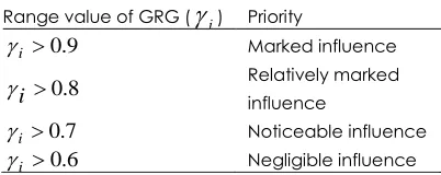
is the value of GRG which indicates the level of the correlation between the reference series and the comparability series [21]. The value of GRG is equal to one if the two series are alike.Table 1 Range of priority list based on GRG values Range value of GRG (
i) Priority9
.
0
i
Marked influence8 . 0
i
Relatively markedinfluence
7
.
0
i
Noticeable influence6
.
0
i
Negligible influenceGenerally, if the value of GRG is more than 0.9, it is indicated as marked influence, more than 0.8 specify as relatively marked influence, more than 0.7 indicates a noticeable influence and more than 0.6 specify as negligible influence. Commonly, if the value of GRG is less than 0.6, it will be removed because it is considered as less importance factors to the reference series [21, 22].
3.2. Support Vector Machine (SVM)
Support Vector Machine is a state-of-the-art learning machine which has been extensively used as a classification tool and found to have a great deal of success in many applications. SVM was proposed by Vapnik et al., [31] based on the statistical learning theory and structural risk minimization principle. SVM first maps the input patterns into a high-dimensional feature space and finds a separating hyper plane that maximizes the margin between two classes [33]. For cancer classification, the classes are divided into benign and malignant tumours. The goal of SVM classification is to produce a model (based on the training data) which predicts the target values of the test data given only the test data attributes. To facilitate this discussion, a brief review of SVM is given in this section.
Consider N pairs of training samples
:
x
i,
y
i
,
i1,2,...n (7)where n
i
R
x
is a real-valued k-dimensional featurevector and
y
i
1
,
1
is the class label ofx
i. A separating hyper plane in the feature space can be described as0 .xb
w (8)
where w is an orthogonal vector and b is a scalar. When the training samples are linearly separable, SVM generates the optimal hyper plane that separates the two classes with maximum margin and no training error [33, 34]. The hyper plane is placed midway between the two classes to maximize the margin [35]. Maximizing the separating margin is equivalent to maximize the minimum value of signed distance d (i) from a point
x
i to the hyper plane [36, 34]. The valueof d (i) can be obtained by
w b x w i
d() . i (9)
The parameter pairs of w and b that corresponding to the optimal hyper plane is the one that minimizes
2
2
1
)
(
w
w
L
(10)subject to
w
x
b
i
n
y
i.
i
1
,
1
,
2
,...
(11)For linearly no separable cases, there is no hyper plane that is able to classify every training point correctly [34]. In order to solve the imperfect separation, the optimization idea can be generalized by introducing the concept of soft margin [36]. Thus, the new optimization problem becomes:
Minimize
N
i
i
C
w
w
L
1
2
2
1
,
(12)so that
wxi b
i i n iy . 1
, 1,2,... (13)where
i is called as slack variables which relates to the soft margin, andC
is the tuning parameter usedto balance the margin and the training error. Both optimization problems in (11) and (13) can be solved using the Lagrange multipliers
i that transform to quadratic optimization problem. According to the Kuhn Tucker theorem of optimization theory [37], the optimal solution satisfies
w
x
b
i
n
y
i ii
.
.
1
0
,
1
,
2
,...
(14)(14) has non-zero Lagrange multipliers if and only if the points
x
i satisfy
.
1
.
w
x
b
y
i i (15)These points are called Support Vector (SV) which lies either on or within the margin. Hence, if
i is the non-zero optimal solution, the classification phase can be stated as
n
i
i
y
i
x
i
x
b
x
f
1
.
sgn
(16)For the application where linear SVM does not produce satisfactory performance, non-linear SVM is suggested. The function of non-linear SVM is to map the feature vector,
x
by a non-linear mapping
x
,implicitly embedded. The kernel function can be explained as
xi xj
xi
xj
k .
.
(17)Where
x
i and
x
j are the inner product of thevectors. The most commonly used kernel functions is the Radial Basis Function (RBF).
2 2
2
exp
.
j i ji
x
x
x
x
k
(18)where
is the parameter controlling the width of the kernel and the Polynomial Function
pj i j
i
x
x
x
x
k
.
.
1
(19)where the parameter,
p
is the polynomial order.3.3. The Proposed Hybrid Method, GRA-SVM
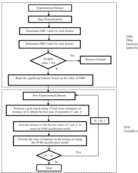
The proposed approach GRA-SVM is classified as hybrid method that combines GRA and SVM. Both models are sequentially implemented and have different purposes. Figure 1 shows the framework of the proposed approach which consists of two main phases: Filter feature selection and Classification.
In feature selection phase, GRA acts as filter feature selection that filters the features based on their priority. The importance of each feature is calculated and ranked based on GRG value. Typically, GRA will select the top ranked features or use a threshold to exclude the irrelevant features. The threshold value used is 0.6 [21]: means that the feature that has GRG value less than 0.6 will be excluded from the list. However, the selected top ranked features may not be the optimal number of significant features candidates.
Therefore, in this study, the selected top ranked features will be selected and evaluated again using SVM. Here, SVM will act not only as classifier to classify the benign and malignant correctly but also plays the role as wrapper feature selection in finding the optimum number of features subset for obtaining the highest classification accuracy. The SVM will do the forward sequential searching for the optimal feature subset by adding a single feature (the most significant features) at a time until the specified criteria is satisfied. In other words, the addition of any features will be continued until
(i) there is no improvement in SVM classification accuracy performance or
(ii) some given bound of is reached, for example, the maximum numbers of the top selected ranked features.
In this case, the second rule is used as stopping criterion. Then, the performance of each subset will be
compared and the best optimum subset is determined based on the highest accuracy classification.
Basically, there are two advantages yield by combining GRA and SVM. First, it can improve the classification performance of GRA as filter method by including learning algorithm in the selection procedure Second, it can increase the efficiency of SVM as classifier in terms of learning time by narrowing the searching space; deleting the irrelevant features will reduce the data dimension.
Figure 1 Proposed GRA-SVM model
4.0 EXPERIMENTS
This section will explain all the experiments that have been carried out during this study.
4.1 Data Description and Data Division
The performance of the proposed method was tested and evaluated using two different types of cancers datasets, breast cancer and liver cancer. These datasets contain the samples of the benign and malignant tumours. The aim of this classification is to classify the benign and malignant tumours correctly using GRA as feature selection with SVM classifiers (GRA-SVM). Both of the datasests are obtained from the UCI Machine Library Database. The summary for both datasets is shown in Table 2.
The breast cancer dataset which is Wisconsin Breast Cancer Database (WBCD) is given by W.Nick Street
GRA Filter Feature Selectio n
SVM Classification
Experimental Dataset
Rank the significant features based on the value of GRG
N = 1,…,m (m = total significant features)
Remove Feature Determine GRG value for eachfeature
Determine GRC value for each feature Data Normalization
Yes
N
o
If GRG value < 0.6
No New Experimental Dataset
Perform a grid search using 3-Fold cross validation on training set to obtain the best pairof parameter C and
N = N+1 Train the training set with the best values of C and to
create the SVM classification model
Classify the class of tumours in the testing set using the SVM classification model
N < m
Yes
(1995) from University of Wisconsin. The dataset consist of 683 samples excluded missing values. These samples were divided into two classes: 444 benign tumours and 239 malignant tumours. There are nine features in the data set which are based on physical appearance of the tumours such as clump thickness, uniformity of cell size, uniformity of cell shape, marginal adhesion and single epithelial cell size of the breast cancer dataset.
For liver cancer, the BUPA Liver Disorders dataset is obtained from BUPA Medical Research Limited is used. The dataset was provided by Richard S.Forsyth in 1990. The total sample data is 345 of which 200 are benign tumours and 145 are malignant tumours. Each data has six features that are based on the blood tests and the level of alcohol consumption.
The breast cancer dataset which is Wisconsin Breast Cancer Database (WBCD) is given by W.Nick Street (1995) from University of Wisconsin. The dataset consist of 683 samples excluded missing values. These samples were divided into two classes: 444 benign tumours and 239 malignant tumours. There are nine features in the data set which are based on physical appearance of the tumours such as clump thickness, uniformity of cell size, uniformity of cell shape, marginal adhesion and single epithelial cell size of the breast cancer dataset.
For liver cancer, the BUPA Liver Disorders dataset is obtained from BUPA Medical Research Limited is used. The dataset was provided by Richard S.Forsyth in 1990. The total sample data is 345 of which 200 are benign tumours and 145 are malignant tumours. Each data has six features that are based on the blood tests and the level of alcohol consumption.
In classification process, each of the datasets is divided into two partitions with the ratio of 70:30. 70% of the dataset is used for training and the other 30% dataset is used for testing. For example, in WBCD data set, from 683 data, 478 of them are used as training data. In addition, another 205 data are used as testing data to test the capability of SVM to classify correctly data that never been used during the training phase.
4.2 Implementation of the Proposed Hybrid Model, GRA-SVM
In this study, the Grey Relational Analysis (GRA) and Support Vector Machine (SVM) methods are combined to improve the capability of SVM as classifier by removing the irrelevant features that can decrease the SVM’s classification precision. The proposed GRA-SVM is implemented in two phases sequentially. Filter feature selection is implemented using GRA and then followed by SVM classifier.
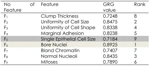
GRA analyzes the influential factor of comparability series to the reference series based on the GRG value [30]. The features of WBCD and BUPA dataset are considered as comparability series while the class of tumours for both datasets (benign or malignant) is stated as the reference series. Table 3 and Table 4 show the GRG value for each feature in both datasets. The higher the value of GRG, presents the most influence features for each dataset. There are no
features considered for elimination as the value of GRG for all features are above 0.6. Thus, as shown in Table 3, the most influential features based on GRA in WBCD dataset are as follows: F6, F2, F8, F3, F4, F9, F7, F1, F5. The result shows that F6 (bore nuclei) is the most important feature that affect the breast cancer while F5 (single epithelial cell size) is the least significant feature that influence the capability of breast cancer occurrence.
While for the BUPA dataset (Table 4), the rank of the features from high to low are, H5, H6, H3, H4, H2, H1. The result indicates that more attention should be given to feature H5 (gammagt) since it has the highest GRG value and the most influential factor that contribute to the Liver cancer. While, H5, H6, H3, H4, and H2 are the moderate influence factors that affect the Liver cancer.
Table 2 The Summary of Cancer Datasets
Type of Canc er
Name of
Dataset Number of Sample s
Numbe r of Feature s
Benign Tumour s
Maligna nt Tumours
Breast Wisconsi n Breast Cancer Dataset (WBCD)
683 9 444 239
Liver BUPA Liver Disorder s
345 6 200 145
Table 3 GRG value of WBCD dataset features
No of
Feature Feature GRG value Rank
F1 Clump Thickness 0.7248 8
F2 Uniformity of Cell Size 0.8475 2
F3 Uniformity of Cell Shape 0.8338 4
F4 Marginal Adhesion 0.8238 5
F5 Single Epithelial Cell Size 0.7184 9
F6 Bore Nuclei 0.8925 1
F7 Bland Chromatin 0.7407 7
F8 Normal Nucleoli 0.8435 3
F9 Mitoses 0.7890 6
Table 4 GRG value of BUPA dataset features
No of Feature Feature GRG value Rank
H1 mcv 0.6719 6
H2 alkphos 0.6908 5
H3 sgpt 0.7325 3
H4 sgot 0.6989 4
H5 gammagt 0.7403 1
Table 5 The nine feature subsets for WBCD dataset
Feature
Subset No Features of Selected Features
X1 1 F6
X2 2 F6, F2
X3 3 F6, F2, F8
X4 4 F6, F2, F8, F3
X5 5 F6, F2, F8, F3, F4
X6 6 F6, F2, F8, F3, F4, F9
X7 7 F6, F2, F8, F3, F4, F9, F7
X8 8 F6, F2, F8, F3, F4, F9, F7, F1
X9 9 F6, F2, F8, F3, F4, F9, F7,
F1, F5
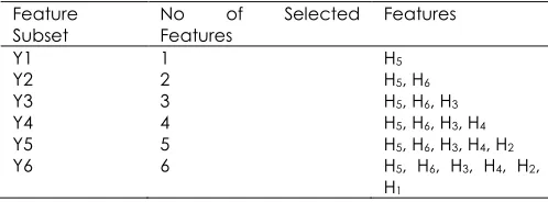
Table 6 The six feature subsets for BUPA dataset
Feature
Subset No Features of Selected Features
Y1 1 H5
Y2 2 H5, H6
Y3 3 H5, H6, H3
Y4 4 H5, H6, H3, H4
Y5 5 H5, H6, H3, H4, H2
Y6 6 H5, H6, H3, H4, H2,
H1
The output of GRA which is the selected features ranked according to GRG value is then used as the input for the SVM classification process. The SVM classification process begins with only one feature which has the highest value of GRG. Then, each time the classification process is repeated, the features are added one by one based on the rank of GRG value until all selected features are used. The feature which has the lowest value of GRG is added last. The sets of features formed are then called feature subsets. Each feature subsets has different number of features. Thus, there are nine feature subsets for WBCD datasets (X1 to X9) and six feature subsets (Y1 to Y6) for BUPA dataset being constructed to build the SVM classification model (refer Table 5 and Table 6).
Besides the right number and appropriate features used as input, the SVM classification accuracy can also be improved through proper parameters setting. There are two parameters need to be considered for optimization RBF kernel function. They are the regularization parameter, of which C determines the tradeoff cost between minimizing the training errors and kernel function parameter, and
defines the non-linear mapping from the input space to some high dimensional feature space. The grid search approach is employed since it is an efficient way to find the best C and
. The range of parameter C and
considered in this study is log2C
1,0,...,3
andlog2
4,3,...,2
. To improve thegeneralization ability, grid search uses a cross-validation process [2]. In grid search, pairs of
C, are tried and the one with the best cross-validation accuracy is chosen. In this study, 3-fold cross validationtechnique is applied on the training set to find the best pairs of
C, . The best values of parameter C and
is then used to create a SVM classification model to train the dataset. The SVM classification model is then implemented to classify the class of tumours in the testing set. Table 7 and Table 8 show the best pair of parameters C and
for each feature subset of WBCD and BUPA dataset.4.3 Performance Measure
The performance of GRA-SVM is evaluated by the percentage of accurately assigned new samples of cancer data to the correct class such as benign and malignant. Benign indicates non-cancerous tumours while malignant indicates cancerous tumours. There are several measuring tools that can be used to evaluate the performance of the proposed classification model such as sensitivity, specificity, accuracy and Area under Curve (AUC) value. Each of them is used to measure different aspects of GRA-SVM performance.
Sensitivity is a measuring tool used to calculate the percentage of correctly classified benign tumours data. Sensitivity is defined as follows [38,39,50]:
Sensitivity (%) =
100
TP
FN
TP
(20)Specificity is the percentage of correctly classified malignant tumours data. Specificity is calculated as follows [33, 40]:
Specificity (%) =
100
FP
TN
TN
(21)
Accuracy approximates how effective the proposed model is by showing the percentage of the true value of the class label. The higher value of accuracy means that the method can accurately classify both types of the tumours. It is given by [41,42,43,44]:
Accuracy (%) =
100
FP
TN
FN
TP
TN
TP
(22)
AUC represents a common measure of sensitivity and specificity over all possible thresholds. The AUC value of 100% represents perfect discrimination (the classifier can classify the tumours correctly), whereas an AUC value of 50% is equivalent to random model. AUC is calculated as follows [6]:
AUC (%) = 100
2 1
TN FP
TN
FN TP
TP
(23)
Although there are many measuring tools which can be used to evaluate the performance of the method but usually most of the researchers chose to determine the performance based on the on the accuracy value [41, 42,49].
5.0
RESULTS AND DISCUSSION
In this section discussion on results obtained from the experiment are presented and discussed.
5.1. Results for WBCD Dataset and BUPA Dataset
Table 9 and Table 10 show the result obtained for WBCD and BUPA dataset using GRA-SVM. As it can be seen from Table 9, for WBCD, GRA-SVM has the highest value of accuracy, sensitivity and AUC; 99.02%, 98.75% and 99.38% using only 2 features (X2). This feature subset, X2 achieved 100% for sensitivity.
It can be said that these two features namely; bore nuclei and uniformity of cell size are the most important features that influence the breast cancer. The patient can be detected having breast cancer or not by looking at these two features only. Therefore, it can facilitate the process and reduce the processing time taken by medical expert in diagnosing the existence of malignant tumours of breast cancer. Furthermore, the integration of GRA and SVM has increase the capability of SVM to detect the breast cancer benign and malignant tumours more precisely. GRA helps to recognize and remove the irrelevant features that affect the SVM classification performance.
Table 7 The best pairs of parameters C and
for WBCD datasetFeature Subset No of Selected
Features C
X1 1 21 2-4
X2 2 20 20
X3 3 2-1 2-1
X4 4 2-1 2-2
X5 5 2-1 2-2
X6 6 20 2-3
X7 7 20 2-4
X8 8 20 2-4
X9 9 20 2-4
Table 8 The best pairs of parameters C and
for BUPA datasetFeature Subset No of Selected
Features C
Y1 1 23 2-4
Y2 2 23 2-4
Y3 3 2-1 2-4
Y4 4 20 2-4
Y5 5 20 21
Y6 6 20 20
Table 9 The value of performance measure for each model of WBCD dataset
Model Accuracy(%) Sensitivity(%) Specificity(%) AUC (%)
X1 92.20 96.25 77.78 87.01
X2 99.02 98.75 100.00 99.38
X3 98.54 98.13 100.00 99.06
X4 98.54 98.13 100.00 99.06
X5 98.05 97.50 100.00 98.75
X6 98.54 98.13 100.00 99.06
X7 98.54 98.13 100.00 99.06
X8 98.54 98.13 100.00 99.06
X9 98.54 98.13 100.00 99.06
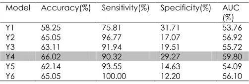
Table 10 The value of performance measure for each model of BUPA dataset
Model Accuracy(%) Sensitivity(%) Specificity(%) AUC (%)
Y1 58.25 75.81 31.71 53.76
Y2 65.05 96.77 17.07 56.92
Y3 63.11 91.94 19.51 55.72
Y4 66.02 90.32 29.27 59.80
Y5 62.14 93.55 14.63 54.09
Y6 65.05 100.00 12.20 56.10
For BUPA dataset (refer Table 10), GRA-SVM achieved the highest result in accuracy (66.02%) and AUC (59.80%) by using only four features (Y4) which are gammagt, drinks, sgpt and sgot. However, the sensitivity and specificity values of Y4 are 90.32% and 29.27% respectively are not the highest among the feature subsets employed in this study.
For example, the specificity of Y1 is greater than Y4. Meaning that Y4 cannot beat Y1 in terms of specificity, but Y4 is better than Y1 in terms of AUC. AUC presents the global performance of the associated features as well as the trade-off between the sensitivity and specificity. Here, AUC is used to estimate the discriminative capability of each feature, for which classifier needed to be generated. Therefore, based on the result obtained, Y4 has larger AUC than Y1. This result indicates that selected features in Y4 have a better classification performance than features in Y1. Furthermore, the accuracy of Y4 is the best. Therefore, Y4 is chosen since it has the ability to classify the benign and malignant more appropriately.
To summarize from the result obtained, there are two important features namely bore nuclei and uniformity of cell size that influence the classification accuracy of breast cancer. While for liver cancer, there are four features shown that the most informative features for classifying liver cancer. Therefore, this information gives important clue to physician or medical expert in assisting to focus on which features that are dangerous and more harmful to the cancer patient.
5.2. Comparison of GRA-SVM with SVM
GRA-SVM (used only selected features) while Figures 2 and 3 show the relation between the number of features and the performance of GRA-SVM and SVM in all measuring tools for WBCD and BUPA dataset.
For WBCD dataset, X9 represents the feature subsets that used standard SVM with 9 features while X2 is the feature subsets that used GRA-SVM with only two features. As can be seen from Table 11, SVM classified WBCD with the accuracy, sensitivity and AUC of 98.54%, 98.13% and 99.06% respectively using nine features, whereas GRA-SVM had the same classification process with 99.02% accuracy, 98.75% sensitivity and 99.38% AUC using only two features. Both models achieved 100% in specificity.
Compared to SVM, GRA-SVM with 77% feature reduction has successfully improves the classification accuracy of SVM classifier in the breast cancer data from 98.54% to 99.02% and increases the SVM classifier sensitivity and AUC from 98.13% and 99.06% to 98.75% and 99.38% respectively.
Figure 2 shows that the values of accuracy, sensitivity and AUC increased when fewer features are used. This result shows that the combination of GRA and SVM for obtaining the optimum feature subsets has successfully increased the SVM classification performance. The capability of GRA-SVM to recognize and remove the irrelevant features which affect the stability of the SVM classifier is beneficial in terms of accuracy performance and reducing the computational cost.
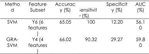
For BUPA dataset, Y6 symbolizes the feature subsets that used SVM with 6 features while Y4 is the feature subset that used GRA-SVM with only 4 features. Table 12 shows that GRA-SVM classified BUPA dataset with 66.02% accuracy, 29.27% specificity and 59.80% AUC while the accuracy, specificity and AUC of SVM using all features are 65.05%, 12.2 % and 53.76% respectively.
Table 11 The comparison of SVM and GRA-SVM for WBCD dataset
Metho
d Feature Subset Accuracy (%) Sensitivity (%) Specificity (%) AUC (%) SVM X9 (9
features )
98.54 98.13 100 99.0 6
GRA-SVM featuresX2 (2 )
99.02 98.75 100 99.3 8
Table 12 The comparison of SVM and GRA-SVM for BUPA dataset
Metho
d Feature Subset Accuracy (%) Sensitivit y (%)
Specificit y (%) AUC (%)
SVM Y6 (6 features
)
65.05 100 12.20 56.1 0
GRA-SVM featuresY4 (4 )
66.02 90.32 29.27 59.8 0
Compared to Y6, Y4 has lower sensitivity but higher specificity. Since the purpose of the cancer detection is to diagnose whether the patient has cancer, which is represented by the existence of malignant tumor; higher precision in specificity is more important in this study. Patients that are detected with cancer can be further investigated to prolong their survival but patients that are classified as normal will remain undetected. Therefore, the capability of classifier to classify correctly the malignant tumor is more important than benign tumor. For this reason, Y4 or GRA-SVM is chosen because its ‘specificity is higher than Y6.
Figure 3 shows that the values of accuracy, specificity and AUC are better when fewer features are used. The result shows that GRA-SVM outperformed SVM as classifier and indicates that feature selection is needed to help the classifier remove the irrelevant features that affect its performance. GRA-SVM hasincreased the performance of SVM classifier and reduced the number of features in SVM about 33.3%.
From the experimental results, they demonstrate that the comparative experiment conducted on the top ranked selected features by the proposed model, GRA-SVM has outperformed the whole features used in SVM in terms of accuracy, specificity, sensitivity and accuracy.
These results indicate that the application of GRA as feature selection has successfully identified and removed the appropriate irrelevant features that can affect the performance of SVM as classifier
5.3. Comparison of GRA-SVM with Previous Methods
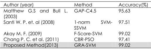
To further validate the performance of GRA-SVM, comparisons with previous methods are carried out. Tables 13 and 14 demonstrate the accuracy performance produced by GRA-SVM and the accuracy obtained from the previous hybrid model that combined feature selection and classifier on both WBCD and BUPA datasets.
For WBCD dataset, the GRA-SVM performance is compared with Genetic Algorithm-Programming with C4.5 (GAP-C4.5), 1-norm SVM with Smooth SVM, F-Score with SVM and Case Based Reasoning with Particle Swarm Optimization (CBR-PSO) methods. Meanwhile, for BUPA dataset, the performance of GRA-SVM is compared with Ordered Fuzzy ARTMAP (O.F.ARTMAP), Bayesian Network Naïve Dependence (BNND), GAP-C4.5, and generalized regression neural network (GRNN).
capability of GAP, 1-norm SVM, F-Score and CBR as feature selection since it can increase the accuracy performance and reduce the number of features employed.
Figure 2 Relationship between the number of features and the performance of SVM and GRA-SVM for WBCD
Figure 3 Relationship between the number of features and the performance of SVM and GRA-SVM for BUPA
For BUPA dataset, as shown in Table 14, the performance of the proposed GRA-SVM is better compared to others. It has the highest classification accuracy of 66.02% which indicates that GRA-SVM has better capability as classifier.
From the results obtained, it can be concluded that the proposed hybrid model, GRA-SVM that combine SVM and GRA as feature selection can produce more reliable and better classification performance in classifying the breast cancer and liver cancer dataset.
Table 13 Performance of GRA-SVM and other methods on the WBCD dataset
Author (year) Method Accuracy(%)
Matthew G.S and Bull L.
(2003) GAP-C4.5 95.63
Santi W. P. et. al (2008) 1-norm
SVM-SSVM 97.51
Akay M. F. (2009) F-Score-SVM 99.02 Chang P. C. et al. (2011) CBR-PSO 97.41 Proposed Method(2013) GRA-SVM 99.02
Table 14 Performance of GRA-SVM and other methods on the BUPA dataset
Author (year) Method Accuracy (%)
Ahluwalia M. and Bull L. (1999) O.F ARTMAP 57.01
Cheung N. (2001) BNND 61.83
Matthew G.S and Larry B. (2003) GAP-C4.5 65.97 Yalcyn M. et al. (2003) GRNN 65.55 Proposed Method (2013) GRA-SVM 66.02
6.0 CONCLUSION
This study has explored a new hybrid model called GRA-SVM for breast cancer and liver cancer diagnosis. The performance of GRA-SVM is tested on two important medical datasets, Wisconsin Breast Cancer Database (WBCD) dataset and BUPA Disorder dataset. To access the effects of feature selection on GRA-SVM classification accuracy, comparison with standard SVM (without feature selection) is carried out using four performance measures: accuracy, sensitivity, specificity and AUC. The result obtained from this study shows that the proposed GRA-SVM has outperformed SVM classifier in all measurement performances by using fewer features that will speed up the training time and decrease the computational time.
Besides improving the classification accuracy, the GRA-SVM also produced a ranking scheme that ranked the features based on their priority. This ranking scheme is very useful since it provides the information to the physician on which features are most dominant that can influence the cancer data. Therefore, the physicians should focus more on these top ranked features to assist them in making accurate decision on cancer diagnosis.
Comparison with the previous studies also shows that the hybridization of GRA and SVM has outperformed the previous hybrid methods in terms of classification accuracy. These results show that the selected feature subset was identified to be most informative by combination of GRA-SVM based reduction approach. Therefore, it is worthwhile for the medical expert to pay more attention to these features when they conduct the diagnosis.
Acknowledgement
This study is supported by the Fundamental Research Grant Scheme (FRGS vot : 4F738) that sponsored by Ministry of Higher Education (MOHE). Authors would like to thank Research Management Centre (RMC) Universiti Teknologi Malaysia, for the research activities and Soft Computing Research Group (SCRG) for the support and motivation in making this study a success
References
[1] Polat K, Sahan S, Kodaz H, Gunes S. 2007. Breast Cancer
And Liver Disorder Classification Using Aritificial Immune Recognition System (AIRS) With Performance Evaluation By
Fuzzy Resource Allocation Mechanism. Expert System Appl.
32:172-183
[2] Akay M. F. 2009. Support Vector Machine Combined With
Feature Selection For Breast Cancer Diagnosis. Expert
System Appl. 36(2): 8-16
[3] Alireza 0, Bita S. 2010. Machine Learning Techniques To
Diagnose Breast Cancer. In: Fifth International Symposium
on Health Informatics and Bioinformatics. 114-120
[4] Chen H. L, Yang B, Wang G, Wang S. J, Liu J, Liu D. Y. 2011.
Support Vector Machine Based Diagnostic System For
Breast Cancer Using Swarm Intelligence. Journal of Medical
System. 36(4): 2505-2519
[5] Pan S. M, Lin C. H. 2010. Fractal Features Classification For
Liver Biopsy Images Using Neural Network-Based Classifier. In: International Symposium on Computer, Communication,
Control and Automation. 227-230
[6] Quinlan J .1996. Improved Use Of Continuous Attributes In
C4. 5. J Artif Intell Res. 4: 77–90
[7] Wu Y, Wang N, Zhang H, Qin L, Yan Z, Wu Y. 2010.
Application Of Artificial Neural Networks In The Diagnosis Of
Lung Cancer By Computed Tomography. In: Sixth
International Conference on Natural Computation.147-153
[8] Makinaci M., 2005. Support Vector Machine Approach For
Classification Of Cancerous Prostate Regions. World
Academy of Science, Engineering and Technology. 7:
166-169
[9] Polat K., Güneş. S, 2007. Breast Cancer Diagnosis Using Least
Square Support Vector Machine. Digital Signal Processing.
17(4): 694-701
[10] Hamilton H. J., 1996. RIAC: A Rule Induction Algorithm Based
On Approximate Classification.In: International Conference
on Engineering Applications of Neural Networks, IEEE.
125-132
[11] Bennett K, Blue J .1998. A Support Vector Machine
Approach To Decision Trees. In: Neural Networks
Proceedings. 2396–2401.
[12] Scholkopf B, Kah-Kay S, Burges CJ, Girosi F, Niyogi P, Poggio
T.1997. Comparing Support Vector Machines With Gaussian
Kernels To Radial Basis Function Classifiers. IEEE Transactions
on Signal Processing. 45(11): 2758-2765
[13] Pontil M, Verri A. 1998. Support Vector Machines For 3-D
Object Recognition. IEEE Transactions on Pattern Analysis
and Machine Intelligence. 20: 637-646
[14] Wan V, Campbell WM. 2000, Support Vector Machines for
Speaker Verification and Identification. In: IEEE Workshop
Neural Networks for Signal Processing. 775-784
[15] Osuna E, Freund R, Girosi F. 1997. Training Support Vector
Machines: Application To Face Detection. In: Computer
Vision and Pattern Recognition Proceedings. 130-136
[16] Joachims, T. 1999. Transductive Inference For Text
Classification Using Support Vector Machines. In:
International Conference Machine Learning Proceedings.
[17] Hassan R, Hegazy AF, Badr AA. 2010. Optimize Support
Vector Machine Classifier Based On Evolutionary Algorithm
For Breast Cancer Diagnosis. International Journal of
Computer Science and Network Security. 10(12): 85-90
[18] Frohlich H, Chapelle O, 2003. Feature Selection For Support
Vector Machines By Means of Genetic Algorithms. In: 15th
IEEE International Conference on Tools With Artificial
Intelligence. 142-148.
[19] Li F. C, Lung TY, Yeh C. H. 2010. Comparison of Filter
Approaches Based on RVFL Classifier. In: Seventh
International Conference on Fuzzy Systems and Knowledge
Discovery. 234-245.
[20] Sallehuddin R., Mariyam SM., Zaiton SMH. 2010. Grey
Relational With BP_PSO For Time Series Forecasting. In: IEEE
International Conference on Systems, Man and
Cybernetics. 253-258
[21] Nagpal G, Uddin M, Kaur A. 2012. A Hybrid Technique Using
Grey Relational Analysis And Regression For Software Effort
Estimation Using Feature Selection. Int. J. Soft Computing
and Engineering. 1(6): 345-351
[22] Yalcin M, Yildirim T., 2003 Diagnosis Of Liver Disorder By
Artificial Neural Networks (In Turkish). In: IX National
Biomedical Engineering Meeting Proceedings. 293-297.
[23] Matthew GS, Bull L. 2003. Feature Construction And
Selection Using Genetic Programming And A Genetic
Algorithm. EuroGP. 229-237
[24] Santi WP, Rahayu SP, Embong A. 2008. Feature Selection
And Classification Of Breast Cancer Diagnosis Based On Support Vector Machines. IEEE. 293-297
[25] Ahluwalia M, Bull L .1999. Co-Evolving Functions In Genetic
Programming: Classification Using K-Nearest Neighbor. In:
Genetic and Evolutionary Computation Conference.
947-952.
[26] Deng J. L. 1982. Control Problems Of Grey Systems. Systems
and Control Letters. 1(5): 288-294
[27] Mat Deris A, Mohd Zain A, Sallehuddin R. 2013. Hybrid
GR-SVM For Prediction Of Surface Roughness In Abrasive Water
Jet Machining. Meccanica. 253-259
[28] Vapnik V .1995. The Nature Of Statistical Learning Theory.
Springer, New York .
[29] Vapnik V .1998. Statistical Learning Theory. Wiley, New York.
[30] Murat C, Mehmet E, Erkan ZB, Ziya YA. 2009. Early Prostate
Cancer Diagnosis By Using Artificial Neural Networks And
Support Vector Machines. Expert Systems with Applications.
36: 6357-6361
[31] Liu Y, Zheng YF. 2004. FS_SFS: A Novel Feature Selection
Method For Support Vector Machines. In: IEEE International
Conference on Acoustic, Speech, and Signal Processing. 5:
797-800
[32] Chen HL. 2011. A Support Vector Machine Classifier With
Rough Set-Based Feature Selection. Expert System Appl.
38(7): 9014-9022
[33] Bertsekas DP. 1995. Nonlinear Programming. Athena
Scientific, Belmont.
[34] Keyvanfard F, Shoorehdeli MA, Teshnehlab M. 2011. Feature
Selection And Classification Of Breast Cancer On Dynamic Magnetic Resonance Imaging Using ANN and SVM.
American Journal of Biomedical Engineering. 1: 20-25
[35] Subashini TS, Ramalingam V, Palanivel S. 2009. Breast Mass
Classification Based On Cytological Patterns Using RBFNN
and SVM. Expert System Appl. 36(5): 5284-5290
[36] Ren J. 2012. ANN vs. SVM: Which One Performs Better In
Classification Of MCCs In Mammogram Imaging.
Knowledge-Based Systems. 26: 144-153
[37] Azmi MS, Cob ZC. 2010. Breast Cancer Prediction Based On
Backpropagation Algorithm. In: Student Conference on
Research and Development. 164-168
[38] Chu F, Wang L. 2006. Applying RBF Neural Networks to
Cancer Classification Based on Gene Expressions. In:
International Joint Conference on Neural Network.
1930-1934
[39] Liao R, Wan T, Qin Z. 2011. Classification of Benign and
Malignant Breast Tumors in Ultrasound Images Based on
Multiple Sonographic and Textural Features. In: Third
International Conference on Intelligent Human-Machine
[40] Chen A.H, Lin C.H. 2011. A Novel Support Vector Sampling Technique To Improve Classification Accuracy And To Identify Key Genes Of Leukemia And Prostate Cancers. Expert System Appl. 38: 3209-3219
[41] Lee, B.1983. String Field Theory, J. Comput. Syst. Sci. 27: 400–
433, doi:10.1142/S0219199703001026.
[42] Loren, R. and. Benson, D. B. 1983. Deterministic Flow-Chart
Interpretations. J. Comput. System Sci. 27(2, Suppl. 290):
400–433.
[43] Tinkham, M. 1964. Group Theory and Quantum Mechanics.
McGraw-Hill, New York.
[44] Beeson, M. J. 1985. Foundations of Constructive
Mathematics. Springer, Berlin: 210-219
[45] Clark, K. L. 1973. Negations as failure, Logic and Data Bases,
eds. H. Gallaire and J. Winker. Plenum Press, New York. 293–
306.
[46] Tel, T. 1990. Experimental Study and Characterization of
Chaos, ed. Hao Bailin. World Scientific, Singapore. 149-159
[47] Srivastava, J. K.. Bhargava, S. C, Iyengar P. K. ,and Thosar, B.
V. 1983. Advances in Mössbauer Spectroscopy: Applications to Physics, Chemistry and Biology, eds. B. V. Thosar, P. K. Iyengar, J. K. Srivastava and S. C. Bhargava.
Elsevier, Amsterdam. 39–89.
[48] Kolmogorov, A. N. 1957. Théorie générale des sytémes
dynamiques et mécanique classique, Proc. Int. Congr.
Mathematicians, Vol. I, Amsterdam, 1954. North-Holland,
Amsterdam. 315–333.
[49] Dubray, J. J., 2003. Standards For A Service Oriented
Architecture. http:// www.ebxmlforum.org/ articles/
ebFor_20031109.html.
[50] Akehurst, D. H. 2004. Transformations Based On Relations.