Sequential algorithm and numerical analysis on mathematical model for thermal control curing process of thermoset composite materials

78: 4–4 (2016) 39–44 | www.jurnalteknologi.utm.my | eISSN 2180–3722 |

Jurnal

Teknologi

Full Paper

SEQUENTIAL

ALGORITHM

AND

NUMERICAL

ANALYSIS

ON

MATHEMATICAL

MODEL

FOR

THERMAL

CONTROL

CURING

PROCESS

OF

THERMOSET

COMPOSITE

MATERIALS

Norma Alias

_{, Hazidatul Akma Hamlan}

_{, Hamisan Rahmat}

a

_{Department of Mathematical Science, Center for Sustainable}

Nanomaterials (CSNano), Ibnu Sina Institute for Scientific and

Industrial Research, Universiti Teknologi Malaysia, 81310 UTM Johor

Bahru, Johor

b

_{Department of Mathematical Science, Faculty of Science,}

Universiti Teknologi Malaysia, 81310 UTM Johor Bahru, Johor

Article history

Received

25 October 2015

Received in revised form

14 December 2015

Accepted

9 February 2016

*Corresponding author

[email protected]

Graphical abstract

Abstract

To reproduce and improve the efficiency of waste composite materials with consistence and high quality, it is important to tailor and control their temperature profile during curing process. Due to this phenomenon, temperature profile during curing process between two layers of composite materials, which are, resin and carbon fibre are visualized in this paper. Thus, mathematical model of 2D convection-diffusion of the heat equation of thick thermoset composite during its curing process is employed for this study. Sequential algorithms for some numerical approximation such as Jacobi and Gauss Seidel are investigated. Finite difference method schemes such as forward, backward and central methods are used to discretize the mathematical modelling in visualizing the temperature behavior of composite materials. While, the physical and thermal properties of materials used from previous studies are fully employed. The comparisons of numerical analysis between Jacobi and Gauss Seidel methods are investigated in terms of time execution, iteration numbers, maximum error, computational and complexity, as well as root means square error (RMSE). The Fourth-order Runge-Kutta scheme is applied to obtain the degree of cure for curing process of composite materials. From the numerical analysis, Gauss Seidel method gives much better output compared to Jacobi method.

Keywords: Numerical analysis, convection-diffusion heat equation, composite materials, temperature profile and sequential algorithm.

© 2016 Penerbit UTM Press. All rights reserved

1.0 INTRODUCTION

Within the past few years, there has been much researchers attempt towards understanding the properties of thermosets composites materials, and this has gone to them for gaining the acceptance among engineering designers. Composite materials are deliberated as a legal substitute towards relatively more conventional materials, as example, plastics,

ceramics or metals. Besides that, composite materials also known as composition materials or shortened to composites. The materials are built from two or more component of materials with considerably variety of physical or chemical properties. By combining the materials together, new different characteristics from previous individual components could be produced. Due to their beneficial of physical and mechanical possessions, it was very competitive for development

Reproduce and improve the efficiency of waste composite materials

Control temperature profile during curing process

Employing Mathematical Model Of 2D Convection-diffusion

Discretize the mathematical model using FDM

Developing sequential algorithm based on two numerical schemes

of manufacturing processes. On the other hand, composites materials also provide design flexibility since many of them can be moulded into complex patterns. In obtaining the desired of mechanical properties, a proper and appropriate curing process, based on opportunely designed pressure and temperature cycles employing vacuum facility need to be performed [1].

During the curing process of thermosets composites materials, heat transfer and resin flow should be considered. Besides that, to produce thick laminate, a proper cure cycle to decrease temperature overshoot and uniform consolidation must be established while the curing process was carried out [2]. However, there are several difficulties to manufacture the thick thermosetting polymer composites. This is due to their lower thermal behavior and conductivity through the thickness of the materials while the process of heat-up and cool down is carried out.

Based on the facts above, this research focuses on the simulation and mathematical modelling for reproducing and remediation that would reduce costly manufacture of thermosets composite material. By employed same physical and thermal properties of materials from [2-5], this papers determines the simulation of temperature profile and the curing degree for composite materials during its curing process.

2.0 EXPERIMENTAL

In this section, the mathematical model that employed in this study, as well as their parameter involve are describe detailed. Two dimensional model of heat equation from Zulkifle, A.K. and Blest, D., et al [3-4] is employed in this paper to predict and visualize the thermal behavior of curing process for thermosets composite materials. The layer’s arrangement of composite materials are visualize by Figure 1 below.

Figure 1 Set up for n resin and carbon fibre

While, the temperature profile of fibre and resin layers, are governed by the following partial differential equation; 𝜕𝑇𝑓 𝜕𝑡 + 𝑢𝑓 𝜕𝑇𝑓 𝜕𝑥 + 𝑣𝑓 𝜕𝑇𝑓 𝜕𝑦 = 𝐾𝑓(

𝜕2_𝑇 𝑓

𝜕𝑥2+

𝜕2_𝑇 𝑓

𝜕𝑦2)

+Ø𝜌𝑟𝐻𝑅 𝜌𝑓𝑐𝑓 𝜕𝛼 𝜕𝑡, (1) 𝜕𝑇𝑟 𝜕𝑡 + 𝑢𝑟 𝜕𝑇𝑟 𝜕𝑥+ 𝑣𝑟 𝜕𝑇𝑟 𝜕𝑦 = 𝐾𝑟(𝜕 2_𝑇 𝑟

𝜕𝑥2 +

𝜕2_𝑇 𝑟

𝜕𝑦2) +

𝐻𝑅

𝑐𝑟

𝜕𝛼 𝜕𝑡,

(2)

The exothermic rate for degree of cure in Equations (1) and (2) above is employed from [4]

𝜕𝛼

𝜕𝑡 = (𝑐1+ 𝑐2𝛼)(1 − 𝛼)(0.47 − 𝛼),

𝑓𝑜𝑟 𝛼 ≤ 0.3 (3)

𝜕𝛼

𝜕𝑡= 𝑐3(1 − 𝛼) 𝑓𝑜𝑟 𝛼 > 0.3, ₍₄₎

𝑐𝑖= 𝐴𝑖𝑒𝑥𝑝 (

−∆𝐸𝑖

𝑅𝑇 ) , 𝑖 = 1,2,3

The initial degree of cure for Equation (3) is α(x,y,t)=0. The composite materials are assume as fully cured if the theoretical value of α reached values of 1. All parameters involve in the mathematical model are presented as in Table 1 below.

Table 1 Parameters for predicting the thermal profile of composite materials

Parameters Value Remarks 𝐻𝑅 474 J/g=0.474 J/kg Heat of reaction

(resin). 𝐾𝑖=

𝑘𝑖 𝜌𝑖𝑐𝑖, 𝑖 = 𝑟, 𝑓

𝑘𝑟= 1.67 x 10−1W/(m K) 𝑘𝑑𝑓= 2.60 x 101W/(m K)

Thermal diffusivities for resin and saturated fibre layer, while 𝑘_𝑖 is thermal conductivity 𝜌𝑖 Resin =1.26 x 103kg/m3

Saturated fibre=1.79 x 103_kg/m3

Density

𝑐𝑖 Resin=1.26 x 103J/(kg K)

Saturated fibre= 7.12 x 102_{J/(kg K)}

Specific heat capacity

𝐴1 𝐴2 𝐴3

2.101 x 109_min-1

-2.104 x 109_min-1

1.960x 105_min-1

Specific pre-exponential factors

∆𝐸1 ∆𝐸2 ∆𝐸3

8.07 × 104 _{𝐽/𝑚𝑜𝑙} 7.78 × 104 _{𝐽/𝑚𝑜𝑙} 5.66 × 104 _{𝐽/𝑚𝑜𝑙}

Activation energies

𝑅 8.31435 J/Kmol Universal gas constant

3.0 FINITE DIFFERENT METHOD (FDM)

In visualizing the temperature profile of the composite materials during its curing procedure, Finite Different scheme is applied in this studies, as discretizing purposed. As the dimensionalized for both Equations (1) and (2) above was done, a weighted approximation from FDM is applied for their discretizing rule. By neglecting the truncation error, the linear system equation that can formed from the discretization can be simplified as

(𝑇𝑓)𝑖,𝑗𝑘+1− 𝐵𝜃(𝑇𝑓)𝑖−1,𝑗𝑘+1 + 𝐴𝜃(𝑇𝑓)𝑖+1,𝑗𝑘+1

+ 𝐶𝜃(𝑇𝑓)𝑖,𝑗𝑘+1− 𝐵𝜃(𝑇𝑓)𝑖,𝑗−1𝑘+1

+ 𝐴𝜃(𝑇𝑓)𝑖,𝑗+1𝑘+1

= (𝑇𝑓)𝑖,𝑗𝑘 + 𝐵(1 − 𝜃)(𝑇𝑓)𝑖−1,𝑗𝑘

− 𝐴(1 − 𝜃)(𝑇𝑓)𝑖+1,𝑗𝑘

− 𝐶(1 − 𝜃)(𝑇𝑓)𝑖,𝑗𝑘

+ 𝐵(1 − 𝜃)(𝑇𝑓)𝑖,𝑗−1𝑘

− 𝐴(1 − 𝜃)(𝑇𝑓)𝑖,𝑗+1𝑘 + 𝐽1𝑘𝛼𝑖,𝑗𝑘

(5)

and,

(𝑇𝑟)𝑖,𝑗𝑘+1− 𝐵𝜃(𝑇𝑟)𝑖−1,𝑗𝑘+1 + 𝐴𝜃(𝑇𝑟)𝑖+1,𝑗𝑘+1

+ 𝐶𝜃(𝑇𝑟)𝑖,𝑗𝑘+1− 𝐵𝜃(𝑇𝑟)𝑖,𝑗−1𝑘+1

+ 𝐴𝜃(𝑇𝑟)𝑖,𝑗+1𝑘+1

= (𝑇𝑟)𝑖,𝑗𝑘 + 𝐵(1 − 𝜃)(𝑇𝑟)𝑖−1,𝑗𝑘

− 𝐴(1 − 𝜃)(𝑇𝑟)𝑖+1,𝑗𝑘

− 𝐶(1 − 𝜃)(𝑇𝑟)𝑖,𝑗−1𝑘

− 𝐴(1 − 𝜃)(𝑇𝑟)𝑖,𝑗+1𝑘 + 𝐽2𝑘𝛼𝑖,𝑗𝑘

(6)

where,

Δ𝑡𝑢𝑖

2∆𝑥 = 𝑎,

Δ𝑡𝐾𝑖

(∆𝑥)2= 𝑏,

Ø𝜌𝑟𝐻𝑅

𝜌𝑓𝑐𝑓 = 𝐽1

𝐻𝑅

𝑐𝑟 = 𝐽2

and

𝑎 − 𝑏 = 𝐴, 𝑎 + 𝑏 = 𝐵, 4𝑏 = 𝐶

Equation (5) and (6) can be categorized as explicit, implicit and Crank-Nicolson scheme by using different value of weighted parameter, 𝜃. As we already concern, value of weight parameter lies between the ranges of 0 ≤ 𝜃 ≤ 1. The algorithm to be construct are depend on the chosen value of 𝜃. In this study, we choose 𝜃 = 0. Therefore, Equation (5) and (6) can be simplifies as below;

(𝑇𝑓)𝑖,𝑗𝑘+1= 𝐵(𝑇𝑓)𝑖−1,𝑗𝑘+1 − 𝐴(𝑇𝑓)𝑖+1,𝑗𝑘

+ (1 − 𝐶)(𝑇𝑓)𝑖,𝑗𝑘 + 𝐵(𝑇𝑓)𝑖,𝑗−1𝑘

− 𝐴(𝑇𝑓)𝑖,𝑗+1𝑘 + 𝐽1𝑘𝛼𝑖,𝑗𝑘

(7)

and,

(𝑇𝑟)𝑖,𝑗𝑘+1= 𝐵(𝑇𝑟)𝑖−1,𝑗𝑘 − 𝐴(𝑇𝑟)𝑖+1,𝑗𝑘

+ (1 − 𝐶)(𝑇𝑟)𝑖,𝑗𝑘 + 𝐵(𝑇𝑟)𝑖,𝑗−1𝑘

− 𝐴(𝑇𝑟)𝑖,𝑗+1𝑘+1 + 𝐽2𝑘𝛼𝑖,𝑗𝑘

(8)

4.0 NUMERICAL TECHNIQUE IN SOLVING

MATHEMATICAL MODELING

As we have discuss above, in order to solve the mathematical model numerically, some Finite Different scheme has been employed for discretization purpose. To extend this studies, some numerical method under consideration are Jacobi and Gauss Seidel methods. Both method are used to solve the linear system of the mathematical model. Results obtain from both methods will be analyzed and compared. Some explanations of the numerical method are as the subtopic below;

4.1 Jacobi Method (JB).

Jacobi method usually known an algorithm for determining the solutions of a diagonally dominant system of linear system equations. This scheme is named after Carl Gustav Jacob Jacobi (1804–1851). By using this method, an element-based approach is used in solving 𝑥 value, (Ghaffar, Alias, Ismail, Murid, & Hassan, 2009) which is;

𝑇_𝑖(𝑘+1)= 1

𝑎𝑖𝑖(𝑐𝑖− ∑ 𝑎𝑖𝑗𝑇𝑗 (𝑘)

𝑗≠𝑖

) , 𝑖 = 1,2, … , 𝑛 (5)

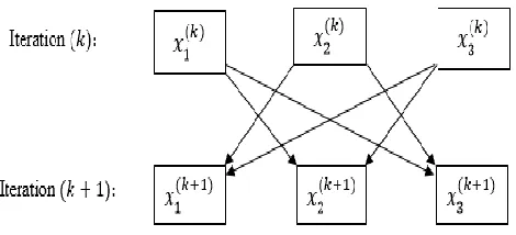
where, k is an iteration number and 𝑎𝑖𝑖≠ 0. Figure 2

below shows the illustration steps of Jacobi method in order to derive the iteration.

Figure 1 Map's calculation for Jacobi Method

4.2 Gauss Seidel Method (GS)

Second iterative method under consideration in this paper for solving the linear system of sequential algorithm is Gauss Seidel (GS) Method. This method is named after Carl Friedrich Gauss (1777-1855) and Philipp L. Seidel (1821-1896). Gauss Seidel method is modified from Jacobi method for solving the linear system. However, this method provide fewer iteration compared with Jacobi method. Calculation using this method are stated as Equation (6) below;

𝑇_𝑖(𝑘+1)= 1

𝑎𝑖𝑖(𝑏𝑖− ∑ 𝑎𝑖𝑗𝑇𝑗 (𝑘)

𝑗>𝑖

− ∑ 𝑎𝑖𝑗𝑇𝑗(𝑘+1) 𝑗<𝑖

) ,

𝑖 = 1,2,3, … , 𝑚

5.0 SEQUENTIAL ALGORITHM

In general, sequential algorithm can be defined as any algorithm that executed sequentially, but, specifically (Daintith, 2004). Illustration of calculation in predicting the temperature profile of composite materials which are resin and fibre layers, can be attained in Figure 3 below.

Figure 2 Sequential algorithm for mathematical model proposed [6,8]

6.0 NUMERICAL ANALYSIS

Based on weight finite difference approximation in Section 3 above, a computer program was develop in order to simulate the thermal profile of composite materials by employing some numerical method which are Jacobi and Gauss Seidel. The platform for this computation was developed and implemented using Microsoft Visual Studio 2013 software with C language. The CPU is supported by Intel® Core-i3 using Windows 8 operating system. However, in this study weight parameter, θ that have been used is 0. It is significant as implicit scheme.

The result comparison between two iterative methods was done by fixing the stopping criteria, which is tolerance at 〖1.0e〗^(-7). However, in this studies, we have plotting the degree of cure using two approach which is using direct method and the second one is using fourth-order Runge-Kutta method. Result simulation for degree cure of both method are visualize in graph form (Figure 4).

(a)

(b)

Figure 3 Visualization of degree of cure vs time using different method a) direct substitution, b) fourth-order Runge-Kutta method

(a)

START

END Initial Condition

Boundary Condition

𝑇𝑘+1_{= 𝑇}𝑘_{+ ∆𝑡}

Numerical Method that considered

Stopping criterion met?

New 𝑇𝑘

Printing the result YES

NO ROUND

(b)

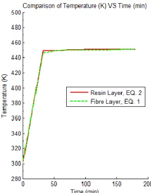
figure 4 Comparison of temperature (k) with time (min) for different method a) jacobi method b) gauss seidel method

For solving the problem in this study, Fourth-order Runge-Kutta method has been used in evaluating the cure degree instead of employing direct method. The main purpose of applying that method is due to its smoothness calculation. As we can observe from Figure 4 above, Fourth-order Runge-Kutta method

could resulting a smooth curve for degree of cure compared with direct method.

Figure 5 (a) and (b) provides comparison between the temperatures and time that computed from the mathematical model with different iterative method approach. Initial temperature used for this experiment

is 300𝐾. The layers of composite materials, which is

resin and fibre layers start to separate from each other when the temperature is different and become constant. From Figure 5 (a) above, it is clearly shows that, the composite materials being apart is around 50 minutes after the experiment was started. While for Gauss Seidel method, that illustrated in Figure 5 (b), the cured of composite materials start as early as around 35 minutes. From the result obtain above, it is obviously seen that, the mathematical model approves well with the numerical solution used.

Result of numerical analysis from iterative method such as the iteration numbers, execution time, the maximum error, computational and complexity also the root means square error (RMSE) are presented in Table 2. Number of iteration can be obtain from the implementation of computer programming while the RMSE is calculate using the formulae below;

𝑅𝑀𝑆𝐸 = √∑ (𝑇𝑘+1− 𝑇𝑘)2

𝑁 𝑖

𝑁

Table 2 Result of numerical analysis for jacobi and gauss seidel methods

NUMERICAL ANALYSIS 𝑁 = 100 𝑡𝑜𝑙 = 1.0𝑒−7

METHODS

Jacobi Method Gauss Seidel Method

EQ 1 EQ 2 EQ 1 EQ 2

Execution time 5.793 sec 5.624 sec 4.927 sec 4.276 sec

Iteration number 99 99 78 78

Computational

Complexity + −

⁄ 10𝑚 10𝑚 10𝑚 10𝑚

× ÷⁄ 18𝑚 15𝑚 18𝑚 15𝑚

Root mean square error 1.4366−3 _2.12568−6 _5.85−4 _2.90258−7 Maximum error 0.040178 0.001501 0.024323 0.000551

Based on Table 2above, the convergence in term of time execution and the iteration numbers between JB and GS methods, showing that, GS method performs faster than JB method. As we can observe from Table 1 above, GS method provides the lowest number of iteration which is 78 as well as give the shortest execution time, which are 4.927 sec and 4.276 secfor Equation (1) and (2) respectively to converge compared with JB method. Number of iteration and computational complexity give a huge impact on execution time of a programming (Alias, Islam, Ahmad, & Razzaque, 2013). Since Jacobi method have a large number of iteration, this resulting the execution time also higher compared to Gauss Seidel method. The judgement of both iterative method above was complete using 1.0𝑒−7 _{tolerance rate and}

𝑁 = 100 data size (size of matrix).

According to (Higham, 2002), the accuracy of an algorithm can be define as relatively or absolutely error of an estimated quantity. In this case, the accuracy of algorithm is measured based on RMSE result. The lowest RMSE would indicates the most accurate method as well as algorithm. Through Table 1 above, the lowest RMSE is belong to Gauss Seidel method. Thus Gauss Seidel method resulting the most accurate result.

7.0 CONCLUSION

employed to solve the linear system of discretization by Finite Different Method.

In order to visualize the thermal profile of curing process for composite materials, numerical method approach can be employed based on the best agreement of graph illustration and result of numerical analysis in Section 6. Numerical analysis for both Jacobi and Gauss Seidel method are compared depend on their number of iteration, execution time, computational and complexity, the maximum error as well as for the root means square error (RMSE).

Based on the numerical analysis that present in Section 6 above, we can conclude that, Gauss Seidel scheme give a better solution compared to Jacobi method in solving Equations (1) and (2) numerically. In future research, it is suggested to employed advance numerical methods such as AGE and IADE for solving the mathematical model. The result can be compared with the basic numerical method that employed in this study.

Acknowledgement

This research is supported in part by the Ministry of Higher Education (MOHE), Research Management Centre (RMC), MYBRAIN15 scholarship and Ministry of Science, Technology and Innovation Malaysia (MOSTI) for the financial support under Research University Grant (08H58). The authors acknowledge the Center for Sustainable Nanomaterials (CSNano), Institute of Ibnu Sina, UTM Johor Bahru for its excellent support for this research.

References

[1]. Carlone, P., D. Aleksendrić, V. Ćirović and G. S. Palazzo. 2014. Modelling Of Thermoset Matrix Composite Curing Process. Key Engineering Materials. 611: 1667-1674. [2]. Oh, J. H. and D. G. Lee. 2002. Cure Cycle for Thick

Glass/Epoxy Composite Laminates. Journal of Composite

Materials. 36(1): 19-45.

[3]. Zulkifle, A. K., 1999. Process modelling of thermoset

composites. Doctoral Dissertation: University of Strathclyde.

[4]. Blest, D., B.R. Duffy, S. McKee and A.K. Zulkifle. 1999. Curing Simulation Of Thermoset Composites. Composites Part A:

Applied Science And Manufacturing. 30(11): 1289-1309.

[5]. Lee, W.I., A.C. Loos and G.S. Springer. 1982. Heat Of Reaction, Degree Of Cure, And Viscosity Of Hercules 3501-6 Resin. Journal of Composite Materials. 13501-6(3501-6): 510-520. [6]. Ghaffar, Z. S. A., N. Alias, F. S. Ismail, A.H.M. Murid And H.

Hassan. 2009.Sequential Algorithm Of Parabolic Equation In Solving Thermal Control Process On Printed Circuit Board.

Malaysian Journal of Fundamental and Applied Sciences.

4(2).

[7]. Daintith, J. 2004. Sequential Algorithm. In a Dictionary of Computing (ed.5). Oxford University Press.

[8]. Alias, N., H. F. S. Saipol and A. C. A. Ghani. 2014. Chronology Of DIC Technique Based On The Fundamental Mathematical Modeling And Dehydration Impact. Journal

Of Food Science And Technology. 51(12): 3647-3657.

[9]. Alias, N., M. R. Islam, T. Ahmad and M. A. Razzaque. 2013. Sequential Analysis of Drug Encapsulated Nanoparticle Transport and Drug Release Using Multicore Shared-memory Environment. Fourth International Conference and Workshops on Basic and Applied Sciences (4th ICOWOBAS) and Regional Annual Fundamental Science Symposium 2013 (11th RAFSS). Johor, Malaysia. 01-06. [10]. Higham, N. J. 2002. Accuracy And Stability Of Numerical

Algorithms. Siam.