ABSTRACT
PHILLIPS, ROBERT. Code Understanding for an Intelligent Tutoring System. (Under the direction of Dr. James C. Lester).
Computer programming is a particularly apt and well-explored domain for Intelligent
Tutoring Systems (ITSs). Central to the success of a programming ITS is the code
understanding system. This thesis explores the possibility of using dynamically constructed
Bayes nets (DCBNs) to understand student coding actions. DCBNs use the observed
evidence to heuristically limit instantiation of the Bayes net to only the relevant portion.
Prior work has applied DCBNs to sketch recognition and story understanding. The
code understanding system described in this work develops heuristics for the domain of
Java code understanding and adds two main extensions to the technique. First, support has
been added for the alteration of prior evidence to allow for student editing of earlier code.
Second, a heuristic has been proposed and tested for the construction of Bayes nets when all
the evidence is not equally informative (e.g., the ―;‖ token is less discriminative than the
―for‖ token).
The DCBN-based code understanding system was evaluated against a top-down
recursive descent parser and a minimum edit distance approach. It was found that, although
the system performed as well as the minimum edit distance baseline and prior DCBN intent
recognition systems (i.e., Wimp3), and could support a fine-grained student model, the
unpredictable behavior, variable execution time and high implementation cost/complexity
Code Understanding for an Intelligent Tutoring System
by Robert Phillips
A thesis submitted to the Graduate Faculty of North Carolina State University
in partial fulfillment of the requirements for the degree of
Master of Science
Computer Science
Raleigh, North Carolina
2011
APPROVED BY:
_______________________________ ______________________________
Dr. James C. Lester Dr. Jon Doyle
Committee Chair
ii
DEDICATION
iii
BIOGRAPHY
Robert Phillips graduated from Harvard University magna cum laude in 1990. He then
pursued a year of post-Baccalaureate studies at Columbia University before joining
Numerical Design Ltd.—a small 3D computer graphics software development firm. While
there, he helped develop the r+ photo-realistic rendering package and the NetImmerse 3D
game engine. In 2003, he joined Applied Research Associates, Inc. and in 2004 began
iv
ACKNOWLEDGMENTS
I would like to thank Dr. Lester for his guidance and assistance throughout the course
of this project. I would also like to thank the other members of the Java Tutor team (Dr.
Kristy Boyer and Michael Wallis) for their help and collaboration. The NCSU IntelliMedia
group has provided a convivial environment for this research and I have greatly benefited
from working with my other group members. Finally, I would like to thank my family for
v
TABLE OF CONTENTS
LIST OF FIGURES ... vii
CHAPTER 1 Introduction... 1
CHAPTER 2 DCBNs for Code Understanding ... 7
Example ... 7
DCBNs for Code Understanding ... 16
Knowledge base. ... 17
Constraints. ... 17
Bayes net construction heuristics. ... 18
The inner loop. ... 20
Bayes net evaluation. ... 24
CHAPTER 3 Evaluation ... 27
Overview ... 27
Corpus ... 27
Baselines. ... 29
Results ... 30
Quantitative. ... 30
Qualitative. ... 52
CHAPTER 4 Related Work ... 55
ITSs for Programming ... 55
LISP tutor. ... 55
Java intelligent tutoring system. ... 56
PROUST. ... 57
Code Understanding... 59
Programmer’s apprentice. ... 59
Plan Recognition ... 60
Wimp3... 60
SketchREAD. ... 61
Knowledge Based Model Construction ... 62
OOBNs and SPOOK. ... 62
Plan to Bayes net conversion. ... 63
Graphical Models ... 64
Bayes nets and decision networks... 64
Dynamic Bayes nets and dynamic decision networks. ... 66
Hidden Markov models... 66
Markov logic networks. ... 67
DCBNs. ... 67
Parsing... 68
Error correcting compilers. ... 68
CHAPTER 5 Discussion ... 70
Results ... 70
vi
Future Work ... 72
CHAPTER 6 Conclusion ... 73
Summary ... 73
Concluding Remarks ... 73
REFERENCES ... 75
APPENDICES ... 81
vii
LIST OF FIGURES
Figure 1. High-level Information flow in an ITS. ... 3
Figure 2. Motivating example of student coding behavior. ... 5
Figure 3. Explanation of Bayes net figures. ... 8
Figure 4. Bayes net after the student types the initial ―a‖ identifier but before pruning. ... 9
Figure 5. Bayes net after the student types the initial ―a‖ identifier and after pruning. ... 10
Figure 6. Bayes net after the student types the ―a‖ identifier and ―=‖ operator but before pruning. ... 11
Figure 7. Bayes net after the student types the ―a‖ identifier and ―=‖ operator and after pruning. ... 12
Figure 8. Bayes net after the student types the ―a‖ identifier, ―=‖ operator and ―0‖ integer literal but before pruning. ... 13
Figure 9. Bayes net after the student types the ―a‖ identifier, ―=‖ operator and ―0‖ integer literal and after pruning. ... 14
Figure 10. Bayes net after the student types the ―a‖ identifier, ―=‖ operator, ―0‖ integer literal and ―;‖ but before pruning. ... 15
Figure 11. Bayes net after the student types the ―a‖ identifier, ―=‖ operator, ―0‖ integer literal and ―;‖ and after pruning... 16
Figure 12: Code Understanding system’s inner loop. ... 21
Figure 13. Development set Programming ... 28
Figure 14. Test set Programming ... 28
Figure 15. Time-scaled Development Data: Mean and standard deviation of evidence. ... 31
Figure 16. Time-scaled Development Data: Comparison of minimum edit and DCBN by fraction of evidence explained. ... 32
Figure 17. Time-scaled Development Data: Fraction of evidence explained for all DCBN sessions. ... 33
Figure 18. Time-scaled Development Data: Minimum edit distance mean and standard deviation of evidence explained fraction. ... 34
Figure 19. Time-scaled Development Data: DCBN mean and standard deviation of evidence explained fraction... 35
Figure 20. Time-scaled Development Data: Number of Bayes net nodes before and after pruning. ... 36
Figure 21. Time-scaled Development Data: Mean and standard deviation of pre-prune number of Bayes net nodes. ... 37
Figure 22. Time-scaled Development Data: Mean and standard deviation of post-prune number of Bayes net nodes. ... 37
Figure 23. Time-scaled Development Data: Pre- vs. Post-pruning maximum number of parents. ... 38
Figure 24. Time-scaled Development Data: Mean and standard deviation of pre-pruning maximum number of parents. ... 39
viii Figure 26. Time-scaled Development Data: Mean and maximum of running time per student
character stroke. ... 40
Figure 27. Time-scaled Test Data: Mean and standard deviation of evidence. ... 42
Figure 28. Time-scaled Test Data: Comparison of minimum edit and DCBN by fraction of evidence explained. ... 43
Figure 29. Time-scaled Test Data: Fraction of evidence explained for all DCBN sessions. . 43
Figure 30. Time-scaled Test Data: Minimum edit distance mean and standard deviation of evidence explained fraction. ... 44
Figure 31. Time-scaled Test Data: DCBN mean and standard deviation of evidence explained fraction. ... 44
Figure 32. Time-scaled Development Data: Number of Bayes net nodes before and after pruning. ... 45
Figure 33. Time-scaled Test Data: Mean and standard deviation of pre-prune number of Bayes net nodes... 46
Figure 34. Time-scaled Test Data: Mean and standard deviation of post-prune number of Bayes net nodes... 46
Figure 35. Time-scaled Test Data: Pre- vs. Post-pruning maximum number of parents. ... 47
Figure 36. Time-scaled Test Data: Mean and standard deviation of pre-pruning maximum number of parents. ... 47
Figure 37. Time-scaled Test Data: Mean and standard deviation of post-pruning maximum number of parents. ... 48
Figure 38. Time-scaled Test Data: Mean and maximum of running time per student character stroke. ... 49
Figure 39. Failed Session: Amount of evidence ... 50
Figure 40. Failed Session: Fraction of evidence explained. ... 51
Figure 41. Failed Session: Pre- vs. Post-Pruned Number of Bayes net nodes. ... 51
Figure 42. Failed Session: Pre- vs. Post-Pruned maximum Number of Parents... 52
Figure 43. Simple Bayes net ... 65
Figure 44. Development Data: Mean and standard deviation of evidence. Non-time-scaled correlate of Figure 15. ... 82
Figure 45. Development Data: Comparison of minimum edit and DCBN by fraction of evidence explained. Non-time-scaled correlate of Figure 16. ... 83
Figure 46. Development Data: Minimum edit distance mean and standard deviation of evidence explained fraction. Non-time-scaled correlate of Figure 18. ... 83
Figure 47. Development Data: DCBN mean and standard deviation of evidence explained fraction. Non-time-scaled correlate of Figure 19. ... 84
Figure 48. Development Data: Number of Bayes net nodes before and after pruning. Non-time-scaled correlate of Figure 20. ... 84
Figure 49. Development Data: Mean and standard deviation of pre-prune number of Bayes net nodes. Non-time-scaled correlate of Figure 21. ... 85
ix Figure 51. Development Data: Pre- vs. Post-pruning maximum number of parents. Non-time-scaled correlate of Figure 23. ... 86 Figure 52. Development Data: Mean and standard deviation of pre-pruning maximum
number of parents. Non-time-scaled correlate of Figure 24. ... 87 Figure 53. Development Data: Mean and standard deviation of post-pruning maximum number of parents. Non-time-scaled correlate of Figure 25. ... 87 Figure 54. Development Data: Mean and maximum of running time per student character stroke. Non-time-scaled correlate of Figure 26. ... 88 Figure 55. Test Data: Mean and standard deviation of evidence. Non-time-scaled correlate of Figure 27. ... 88 Figure 56. Test Data: Comparison of minimum edit and DCBN by fraction of evidence explained. Non-time-scaled correlate of Figure 28... 89 Figure 57. Test Data: Minimum edit distance mean and standard deviation of evidence explained fraction. Non-time-scaled correlate of Figure 30. ... 89 Figure 58. Test Data: DCBN mean and standard deviation of evidence explained
1
CHAPTER 1 Introduction
Human tutoring has a long history in education and has been shown to be very
effective. Bloom’s studies of human tutors (Bloom, 1984) showed expert human tutoring
resulted in excellent learning gains (i.e., tutored students performed two standard deviations
better than control students) and reduced learning differences (i.e., 90% of the tutored
students performed as well as the top 20% of the control students). Additionally, human
tutoring was shown to improve student affect including attitude towards learning, interest and
motivation (Anania, 1983). Unfortunately, human tutoring is expensive and cannot scale
effectively to a large number of students.
Intelligent Tutoring Systems (ITSs) are a product of educational theory, Artificial
Intelligence (AI), and computer-human factors and attempt to provide the benefits of human
tutoring to an unlimited number of students. ITSs have been developed for a wide variety of
domains (e.g., ITSpoke for physics (Litman & Silliman, 2004), AutoTutor for physics and
computer literacy (Graesser, Jackson, Mathews, Mitchell, Olney, Ventura, Chipman,
Franceschetti, Hu, Louwerse, & Person, 2003), CIRCSIM-Tutor for blood pressure (Evens,
Brandle, Chang, Freedman, Glass, Lee, Shim, Woo, Zhang, Zhou, Michael & Rovick, 2001)
and the Geometry Explanation Tutor for mathematics (Aleven, Koedinger & Popescu, 2003))
and have yielded impressive cognitive and affective results. In several studies (Graesser et
2 Wintersgill, 2005; Anderson, Corbett, Koedinger & Pelletier, 1995), ITSs have been shown
to provide about a one standard deviation improvement in learning.
As a subject dear to the hearts of computer scientists, it should not be surprising that
programming has been a popular domain for ITSs. Computer programming is a difficult skill
to acquire, has been well studied educationally, has a wealth of supporting tools and
technology (e.g., parsing tools and development environments) and is in high demand. All
these features make programming an attractive domain for ITSs.
To improve learning and keep students motivated, an ITS (programming or
otherwise) must provide effective interactions with students. To achieve this, ITSs generally
consist of six main components (see Figure 1). First, the natural language understanding
(NLU) module converts student queries to a format the ITS can process. In parallel, for task
oriented domains, the action tracking module interprets student actions, informs the dialog
manager and updates the student model. Next, the dialog manager (DM) interacts closely
with the pedagogical planner and handles conversational pragmatics (e.g., grounding,
adjacency pairs, and so on). The student model represents the student’s knowledge and
emotional state, is usually based on the system’s underlying educational and affective theory
and incorporates the domain knowledge. The pedagogical planning (PP) module monitors the
student’s cognitive and affective state and determines the next most suitable tutorial action.
Finally, the natural language generation (NLG) module generates tutor responses or queries
and is often template-driven. This work will focus on the development and evaluation of the
3
Student Model
NLG DM
PP
NLU Action Tracker Student
Actions
Student Queries
Figure 1. High-level Information flow in an ITS.
A programming ITS’s code understanding system must provide sufficiently detailed
information to allow effective tracking of and response to student actions. In solving this
problem, code understanding systems have generally varied with respect to four main
parameters: the range of accepted input (i.e., how much variability in the student solution is
allowed), the level of interactivity (i.e., token-by-token vs. sub-routine at a time), the
implementation complexity and the granularity of the information provided to the student
model. For example, the PROUST system (Johnson, 1986) supported a wide range of input
in the form of a compileable subroutine but used a complex plan-based recognition system.
LISP Tutor (Anderson & Reiser, 1985), on the other hand, greatly constrained the student’s
input but performed a token-by-token tracking of student actions. It, too, used a very
complex plan-based recognition system, but performed some pre-compilation to accelerate
tracking. Both systems supported a very fine-grained model of the student’s programming
knowledge. From prior observation of human tutors (Boyer, Phillips, Wallis, Vouk, & Lester,
2008), it appears a desirable code understanding system should accept a wide range of input
token-by-4 token tracking of student actions. Ideally, the code understanding system should also be
reasonable to implement and support a fine-grained student model.
As a motivating example, consider the code in Figure 2—a composite of student
errors seen in our training set. Here the student has used a ―while‖ keyword instead of a ―for‖
and replaced the semi-colons with commas. To match human tutoring behavior, a code
understanding system must be able to accept such buggy and incomplete input even though it
isn’t compileable. In the ―while‖ for ―for‖ case, the human tutor often intervened early once
the student began coding the test clause of the for loop. For an ITS to replicate this behavior,
the code understanding system cannot wait until the code is compileable. For the ―,‖ for ―;‖
bug the human tutor would often wait until the student attempted to compile the code before
intervening. To mimic this behavior the code understanding system must be able to ignore
some errors while still providing the most probable interpretation at any given step (e.g.,
5
/**
* Method: plotTimes
* Purpose: Plots the response times on a graph. * Maddie's note: This method needs to go through the * array (arrayToPlot) and pass each element
* to the AmbulanceGUI.plotValue()
* which that takes a double.
* @return This method does not return a value; it
* simply calls a method in the AmbulanceGUI class * to plot the data points
*/
public void plotTimes(double [] arrayToPlot) {
//To-do: Iterate through arrayToPlot. Call the method //AmbulanceGUI.plotValue() on every array element. while(int i = 0, i < 50, i++)
}
Figure 2. Motivating example of student coding behavior.
To meet the desired requirements of a programming ITS’ code understanding system
(i.e., accept a wide range of input, provide token-by-token tracking, be reasonable to
implement and support a fine-grained student model), this thesis explores the use of
Dynamically Constructed Bayes Nets (DCBNs) (Alvarado, 2004). In this approach, as
evidence (i.e., a token) is added, the code understanding system heuristically alters a Bayes
net representing the student’s program. The heuristic construction focuses the
recognition/understanding problem on hypotheses for which there is reasonable evidence (vs.
just trying all hypotheses) while Bayes net inference allows competing hypotheses to
influence each other. This approach promises to support a wide range of input due to the
6 aggressive pruning of the Bayes net. Additionally, the implementation time and complexity
should be similar to other code understanding systems (e.g., PROUST and LISP Tutor),
while higher-level Bayes net hypotheses and the linking of each Bayes net fragment to a
portion of the student’s knowledge should enable a fine-grained student model.
The next section (Chapter 2) will describe the proposed code understanding system.
Chapter 3 will then provide a quantitative and qualitative evaluation of its performance,
while Chapter 4 will cover related work in programming ITSs, code understanding, graphical
models, and compilers. A discussion of the results will follow in Chapter 5 with Chapter 6
7
CHAPTER 2
DCBNs for Code Understanding
This thesis documents the development and implementation of a Java code
understanding system to evaluate the applicability of DCBNs. The developed system
repurposes Alvarado and Davis’ DCBN architecture (Alvarado & Davis, 2005) to support
code understanding instead of sketch recognition. The following discussion will present the
implemented system and point out how it differs from Alvarado and Davis’ approach.
Example
To better illustrate the operation of the DCBN-based code understanding system, the
running example of the student typing the code ―a=0;‖ will be used. The Bayes nets resulting
from each stage in this process are shown in Figure 4 through Figure 11.
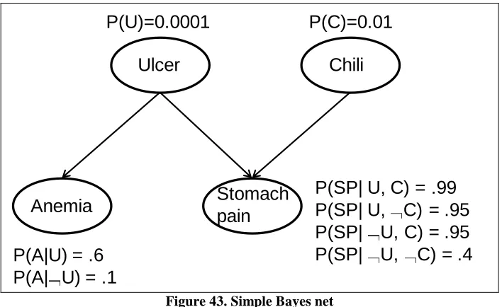
Figure 3 provides a key for interpreting the Bayes nets. Each ellipse represents a
Bayes net node, with the associated label being either the rule name or token it represents.
Below and to the right of each node is listed the probability of the node followed by a colon,
and then if the node is parentless, its prior probability, but if the node is a child, then the leak
probability. This leak probability is used to represent the likelihood that some hypothesis not
present in the Bayes net could have caused the associated node. Each child arrow out of a
node is labeled with the causal strength (i.e., the probability that the parent could cause the
child independent of all other possible causes). Note that the Bayes nets used by the DCBN
system exclusively employ Noisy OR nodes. These canonical causal relations only require
8 reducing the number of probabilities required to fully specify the joint distribution. Finally,
each node is color coded by its probability. Strongly believed nodes are fully saturated green,
while low probability nodes are black.
Figure 3. Explanation of Bayes net figures.
Figure 4 shows the Bayes net after the initial ―a‖ identifier has been added but before
pruning. The ―a‖ token (lower-left corner) has spawned a parent Identifier hypothesis.
Although the Identifier hypothesis has two parents, there are other possible causes that have
not been added to the Bayes net. To compensate for this probabilistically, a leak probability
(0.03) has been added to the Identifier hypothesis. Of the Identifier hypothesis’ two parents,
one is strongly believed (i.e., the idOrClassRef hypothesis with a belief of .71), while the
other is very weak (i.e., the variableDeclaratorId with a belief of .031). In this case, the
weaker hypothesis will be pruned away since it is below a threshold of the stronger
hypothesis’ belief. When the variableDeclaractorId node is pruned away, so too will its
parent and both of their children, since without the variableDeclaractorId node they will all
9 quadrant also has two parents, but since the probabilities are so similar (i.e., .078 and 0.11)
neither one can be pruned away. This likelihood-based pruning can be seen as a harsher form
of the Bayes nets’ explaining away phenomena. If one hypothesis is obviously not a viable
candidate, it is just removed from the net. Figure 5 shows the initial Bayes net after pruning.
The leak probability of the Identifier node does not change since (as will be discussed more
later) parents that are pruned away are not allowed to add their causal strength in absentia.
10 Figure 5. Bayes net after the student types the initial “a” identifier and after pruning.
Figure 6 shows the state of the Bayes net after the ―=‖ operator has been added but
before pruning has occurred. In this Bayes net, the ―=‖ token has spawned an
assignmentOperator hypothesis and a hypothesis that it is part of the optional initialization
portion of a variable declaration (i.e., the ―R75_sub0 node). The assignmentOperator
hypothesis has recursively created an sExpression1Rest hypothesis (i.e., that the assignment
operator is part of an assignment expression). This sExpression1Rest hypothesis is prevented
from recursively generating more hypotheses because one of its required children
(sExpression2) is not supported by any evidence. As in Figure 4, the R75_sub0 hypothesis
will be pruned because its likelihood is far less than its competing parent (i.e., the
12 Figure 7. Bayes net after the student types the “a” identifier and “=” operator and after pruning.
Figure 8 shows the Bayes net after the student has added the ―0‖ integer literal but
before pruning. In this case, the integer literal has completed the sExpression2 hypothesis,
allowing the sExpression1Rest hypothesis to recursively generate parent hypotheses. One of
these parents incorporates the idOrClassRef hypothesis and then continues recursively
generating up to the R159_sub0 level. This hypothesis represents a collection of
blockStatements. Note that while the causal strength for the first blockStatement is 1.0, the
second blockStatement’s causal strength is only .25. This results from the fact that blocks
usually consist of only one or two statements for the selected problem. The causal strengths
are computed from the development portion of the corpus and thus reflect the quick drop off
13 Figure 8. Bayes net after the student types the “a” identifier, “=” operator and “0” integer literal but
before pruning.
Figure 9 shows the Bayes net for ―a = 0‖ after pruning. The node labeled ―; - 0‖ is a
proposed evidence node. Such nodes represent tokens the system believes the student will
type in the future. When the actual semi-colon token is added in Figure 10, it greedily
replaces the proposed evidence, orphaning it. It is pruned away in Figure 11, leaving the final
Bayes net interpretation. In this case, due to the simplicity of the problem and lack of
ambiguity, only the correct abstract syntax tree remains. For a non-toy example, the Bayes
14 Figure 9. Bayes net after the student types the “a” identifier, “=” operator and “0” integer literal and
15 Figure 10. Bayes net after the student types the “a” identifier, “=” operator, “0” integer literal and “;”
16 Figure 11. Bayes net after the student types the “a” identifier, “=” operator, “0” integer literal and “;”
and after pruning.
DCBNs for Code Understanding
Reapplying SketchREAD’s DCBN-based architecture to code understanding required
many modifications. For their sketch recognition domain, Alvarado and Davis used a
hierarchical description of the shapes for their knowledge base, which needed to be changed
to address Java programming. The low-level constraints had to be changed, from the
geometric ones used for sketch recognition to ones more suited to code understanding (e.g.,
17 existing artifact (since students frequently return and alter earlier written code) and to deal
with evidence of varying importance (i.e., the ―;‖ and ‖)‖ tokens are less informative than the
―for‖ and ―if‖ tokens). Finally, SketchREAD’s limitation that shapes cannot be recursive had
to be removed since many programming language grammars require recursion.
Knowledge base. The knowledge base used for the implemented code understanding system is a simplified grammar for the Java language. This grammar was derived from
Parr et al.’s (2006) Java 1.5 grammar and Gosling, Joy, Steele and Bracha’s (2000) partial
Java grammar. The simplified grammar was created by removing productions not required
to parse the development corpus, followed by a reduction of the grammar’s hierarchical
structure (especially with regard to expressions) to reduce the depth of the generated Bayes
net. This simplification step was taken to simplify development of the DCBN algorithm and
reduce its execution time.
The grammatical rules allow the DCBN system to ―understand‖ the student’s code at
the grammatical level. Were this work taken further, PROUST-like intent recognition rules
(e.g., a running-count iterator pattern) would be added to form an additional layer of
hypotheses on top of the grammar-derived ones. Additionally, a layer of student knowledge
rules could be added to map from both the grammatical and intent recognition levels to the
student model. Finally, rules or knowledge derived from the specific problem the students
were solving could then help guide the system’s understanding of the individual problem’s
code.
18 geometric constraints have been replaced with lexical order and lexical distance constraints.
When new evidence or hypotheses are added to the Bayes net, a topological sort (Cormen,
Leiserson, Rivest, & Stein, 2001) is applied, using the parent-child relations and order of the
tokens in the student’s code as constraints. This yields a consistent numbering of all the
nodes in the Bayes net. The numbers from the evidentiary nodes (i.e., tokens) are then
propagated throughout the graph, updating each node’s range of evidentiary support. This
evidentiary support range is used in several ways to reduce the number of combinations
considered in the Bayes net construction process.
Bayes net construction heuristics. Although the core of Alvarado and Davis’ Bayes net construction process remains the same, updating it to the code understanding domain
required several new heuristics to both deal with the new domain and address limitations in
Alvarado and Davis’ approach.
Slot filling. A first alteration in the Bayes net construction process was the use of the
evidence numbering and evidentiary support system to constrain hypothesis generation.
When filling slots in a grammar rule’s hypothesis, the selected slot fillers were
required to have a consistent left to right ordering. This greatly reduced the number of
combinations the Bayes net system needed to consider. It did not eliminate consideration of
the cases where a student transposed two tokens, but instead caused the system to generate
two hypotheses to explain the error—each considering its transposed token to be in the
correct location but with the other token not incorporated.
One issue with the original DCBN system was that whenever the student created an
19 create a new method declaration hypothesis regardless of the separation between the two
tokens. To limit the generation of such implausible hypotheses, the maximum evidence range
of a hypothesis (captured by the number of tokens supporting the hypothesis) was used to
limit the range from which a given parent hypothesis could draw its children. The maximum
range of used evidence was determined for each rule using the development portion of the
corpus. This maximum range was then bloated to allow for some random student insertion
errors (e.g., allowing two additional tokens to the left and right). At run-time, when some
parent hypothesis was being considered for instantiation, the evidence index of the
motivating evidence (i.e., the child node that was driving the parent’s instantiation) was used
to center the parent’s maximum range. Potential candidates to become children of the parent
hypothesis were then selected from only within that range. This heuristic prevented the
parent hypothesis from selecting children an arbitrary distance away in the student’s code.
This was not as restrictive as it seems, since, if ever a hypothesis did require evidence outside
of its range, multiple hypotheses would be created to explain portions of the evidence —a
situation that could be detected and explicitly handled in a more complete system.
Editing existing code. The evidentiary support range and maximum evidence range
were also used to deal with student modifications to existing code. Deletions are well
handled by the existing system, but student insertions can lead to a case where a hypothesis is
no longer plausible because the child nodes have incrementally become too far apart (e.g.,
the student starts with ―a=0;‖ but changes it to ―a=1; b=0;‖). Without some means to remove
the original hypothesis, the Bayes net construction process can get stuck, since the original
20 code understanding DCBN system explicitly checks for hypotheses that have grown beyond
their maximum range and removes them from the Bayes net. This too is not as restrictive as it
sounds, since the top-down step can re-instantiate reasonable hypotheses to explain the data.
Evidence importance heuristic. In both of SketchREAD’s domains, the informational
value of each primitive stroke was relatively constant. For Java this is not true, with many
tokens (e.g., ―;‖, ―(―, ―)‖) being particularly non-informative. An importance-weighting
system was used to prevent all tokens from always generating all their parents.
The development portion of the corpus was used to calculate P(rule | token) for all
rules and tokens. These distributions were then rescaled and thresholded for each rule, so that
only the most determinative of a rule’s children would cause its generation. This
correspondingly means that some tokens (i.e., ―;‖ and ―)‖) never instantiate parent
hypotheses but merely slot into existing hypotheses.
Recursion. Recursion is handled by an explicit check to limit infinite recursion when
the Bayes net is being constructed. The maximum recursion level for each rule is computed
using the development portion of the corpus. That limit is then used to cap the recursion at
run-time. As was mentioned earlier, the grammar was altered (particularly the expression
portion) to reduce the grammar’s reliance on recursion.
The inner loop.The basic algorithm for assembling Bayes nets (see Figure 12) is a four-step process that occurs as each new piece of evidence is received. Each step is geared
towards controlling the potential for combinatorial growth of the Bayes net, while
21
I) Bottom Up Processing
Take new input and incorporate into the Bayes net
II) Top Down Processing
Use Bayes net state to flesh out net
III) Pruning
Heuristically remove hypotheses
IV) Choose Most Likely Interpretation
Figure 12: Code Understanding system’s inner loop.
In Step I, for each key press, the DCBN algorithm spawns a token-level minimum edit
distance pass over the student’s code to find the inserted and deleted tokens. Deleted tokens
simply lose their evidentiary status in the Bayes net and are usually pruned away on the next
pass. For new tokens, the existing proposed evidence (e.g., the ―; - 0‖ node in Figure 9) is
examined to find any that are consistent with regard to their lexical constraints. If a match is
found, the new token greedily replaces the proposed evidence in the Bayes net (e.g., the real
―;‖ replacing the ―; - 0‖ node). If no match is found, then the new token is simply added to
the Bayes net. In either case, every rule that contains the new token in its right hand side is
considered as an explanatory hypothesis. At this point, the P(rule | token) information is used
to skip hypothesis instantiation for non-discriminative tokens. Also at this point, the
maximum evidence range of each proposed hypothesis is computed by expanding the
evidentiary basis of the driving Bayes net node using the proposed rule, token and the token’s
22 rule definition are then used to find all the possible slot fillers for the rule (reserving the
driving Bayes net node’s slot solely for it). Except for the driving Bayes net node’s slot,
instantiating new proposed evidence is also considered. Each possible combination of the slot
fillers is then generated and evaluated based on several criteria.
First, the proposed rule must have sufficient evidence to be instantiated (i.e., taking
into account optional portions of the rule, are there enough evidence-supported children to
warrant the hypothesis’ instantiation). This evidential support test is different from the one
used in SketchREAD. For the parsing domain, a hypothesis is required to have pre-existing
nodes for each slot to the left of the driving Bayes net node (i.e., no proposed evidence is
allowed). This acts to reduce the amount of proposed evidence that is created overlaying the
code the student has already completed. Second, all the children’s evidence constraints must
be consistent and must form a valid left-to-right ordering with no duplication. Third, the
hypothesis cannot cause improper recursion, and finally the hypothesis cannot duplicate an
existing hypothesis. If all these tests are satisfied, then the hypothesis is instantiated.
Care is taken during instantiation to greedily reuse any existing incomplete rule nodes
that are consistent with the child nodes. Additionally, existing Bayes net nodes (particularly
the proposed evidence) are reused as much as possible. These two steps serve to greedily
minimize the Bayes net size.
If, upon instantiation, a rule is completely supported by its children (vs. having
several proposed evidentiary children), the bottom up Bayes net creation process is repeated
on the newly completed node (e.g., the sExpression1Rest node in Figure 8). Because the code
top-23 down pass, when a proposed evidentiary node is replaced with real evidence), the code
understanding DCBN system must also sometimes make a special traversal up the Bayes net,
firing off recursion on Bayes net nodes that have become complete through other means.
This approach to controlling the combinatorial growth of hypotheses is similar to
SketchREAD’s constraint based system (although a bit more rigid). Each hypothesis is
evaluated with regard to the constraints it must satisfy prior to its instantiation. In no case is a
hypothesis added to the Bayes net if it would cause a cycle in the graph.
For Step II of the inner loop of the code understanding domain, the top down step
performs two actions. It attempts to complete any incomplete hypotheses, and tries to replace
proposed evidence with real evidence. The first action operates by finding all the rules for
which an incomplete node is a left hand side. Each candidate is then evaluated in exactly the
same way as in the bottom up step. The second action operates by scanning through the
proposed evidence and the real evidence, checking for a pair whose constraints are
consistent. If such a match is found, the proposed evidence is greedily replaced with the real
evidence.
In SketchREAD, Alvarado and Davis included a re-interpretation pass in their Step II.
This pass would consider alternate interpretations of the user’s strokes given the context
provided by higher-level hypotheses (e.g., could this ―line‖ actually be a poorly drawn
ellipse). This step made sense in the sketch recognition domain where low-level input noise
was common, but was not found useful in the code understanding domain (i.e., it was not
24 For the pruning step (Step III), the code understanding DCBN system implements
SketchREAD’s likelihood and redundancy-based pruning. For the first, all the parents of a
node are compared and those below a threshold of the most likely are removed (as seen in
Figure 4 and Figure 5). Care is taken during the pruning process to ensure that all nodes that
are going to remain keep all of their children, preventing holes from opening up in a
hypothesis. Redundancy-based pruning is implemented via a garbage collection step that
eliminates duplicate hypotheses and merges proposed evidence. This step greatly reduces
clutter in the Bayes net.
In SketchREAD, Alvarado and Davis also implemented an age-based pruning step
where the age of each incomplete hypothesis was compared against some tolerance and those
that were too old were removed. The intuition here was that if the user had not completed a
figure after some time limit, they did not ever intend to do so. Age-based pruning was found
to be inappropriate for the code understanding domain since students would frequently
partially complete a portion of the code and then return to it much later (e.g., begin a for loop
then work on the loop contents then return to fix bugs in the for loop.)
Finally, for the interpretation selection step (Step IV), the code understanding DCBN
selects the single most-likely top-level hypothesis (e.g., a method declaration). This is a bit
stricter than SketchREAD’s system of collecting a set of hypotheses that together cover the
available evidence, but allows direct comparison of the chosen hypothesis with the top-down
recursive-descent compiler’s abstract syntax tree.
25 appropriate probability distributions must be provided, missing/pruned parents need to be
handled and the actual inference method must be selected.
Whereas SketchREAD used a combination of empirically and manually determined
probabilities, all of the code-understanding system’s probabilities were empirically
determined. Both the prior probabilities for each rule and the causal strengths for the Noisy
OR nodes were computed from the development portion of the corpus. In SketchREAD,
Alvarado and Davis set P(child=t | parent=t) to 1.0, if the child were a required portion of the
parent, or to 0.5, if the child were an optional portion of the parent. Although the empirical
method is more accurate, in practice it made a difference in only a few cases (e.g., for
non-uniformly distributed optional nodes – since required children were also empirically always
1.0).
Because the DCBN algorithm only generates a portion of the full Bayes net, it is
necessary to account for the influence of parent nodes that are either not instantiated or have
been pruned away. The code understanding system assumes that parents that have been
pruned away are no longer viable and will not have any influence on their orphaned children.
It constructs a leak probability for each node that takes into account the likelihood that that
node could have been caused as a result of a parent that was not currently in the Bayes net
(and had not been previously pruned away). SketchREAD accounted for missing hypotheses
in the exact same manner.
Finally, to actually perform the Bayes net inference, the code understanding system
used the University of Pittsburg’s Decision Systems Laboratory’s SMILE (SMILE)
26 SketchREAD’s use of loopy belief propagation. It was found that, for the smaller Bayes nets
in the code understanding domain, the relevance-based decomposition was fast enough and
more reliable than loopy belief propagation (please see the evaluation section for more
discussion of this topic). Unlike SketchREAD, the code understanding DCBN system did not
arbitrarily limit the maximum number of parents to eight. It was hoped that this would allow
27
CHAPTER 3 Evaluation
Overview
In order to mimic the observed behavior of human tutors, an ITS must be able to
recognize a student’s intent, even when confronted by partial, buggy and un-compileable
code, and it should be able to perform this recognition in real-time. Additionally, the code
understanding system should be reasonable to implement and maintain and support a
fine-grained student model.
The evaluation of the implemented system will use the above four criteria to assess
DCBN’s suitability for ITS code understanding. Recognition capability will be assessed
through comparison against a recursive descent top-down parser and a minimum edit
distance baseline. For the minimum edit distance comparison, the fraction of available
evidence explained will be used as a metric. The code understanding system’s performance
will be assessed by its processing time per student input character. Code complexity will be
assessed via lines of code and development time. Finally, student model support will be
assessed qualitatively.
Corpus
The corpus used for the evaluation was derived from a series of human-tutor
novice-programmer tutoring sessions. For each session, the tutor and student were only allowed to
communicate via a chat interface and the tutor could see but not alter the student’s coding
28 logged to a database yielding a detailed corpus of student actions and tutor interventions.
This corpus was divided 2/3-1/3 into development and testing portions with 20 sessions
selected for development and 10 for testing.
For development and evaluation purposes only a portion of the tutored problem was
used. Figure 2 shows the method the students had to complete. All students used a for loop to
accomplish the task, but varied in the usage of variables, declarations of the variables and use
of brackets.
Figure 13 and Figure 14 show the number of student programming actions in the
development and testing sessions respectively. The development portion had a mean of 139.0
programming actions (i.e., keystrokes) per session, with a standard deviation of 55.68 while
the testing portion had a mean of 152.7 programming actions per session with a standard
deviation of 56.03. The development portion was compileable 11.4% of the time (i.e., the
student code could be compiled only 1/10 of the time), while the testing portion was
compileable 8.6% of the time. All sessions (both development and testing) ended in a
compileable state.
Figure 13. Development set Programming Action Histogram.
29
Baselines.
Compiler. To assess the code understanding system’s grasp of the student code,
whenever the code is compileable the compiler’s abstract syntax tree is compared to the
Bayes net’s interpretation. In this case, the compiler’s abstract syntax tree represented the
ground truth and comparing the Bayes net’s answer to it assesses whether the Bayes net is
correctly interpreting the student’s code. To make this feasible, the compiler and Bayes net
employ the same grammar.
Minimum Edit Distance. Minimum edit distance was used as the second baseline for
the DCBN code understanding system’s evaluation. Minimum edit distance is a simple and
widely used method for student response evaluation, in which the system matches the student
solution against a set of answers and selects the one that is closest as measured in insertions
and deletions. For the code understanding system’s evaluation, a minimum edit distance
system was implemented that operates at the token level (i.e., it finds token insertions and
deletions rather than character insertions and deletions). The answer key was also specified in
tokens. An identifier in the answer key needed only be matched by another identifier-typed
token in the student’s code to be considered a match. All other tokens (e.g., keywords) must
have matched in both type and contents. This permissive matching scheme corresponds to the
DCBN’s operation (i.e., constraints on identifier values were not added to the Bayes net)
30
Results
Quantitative.
Development set results. The development set was used to implement the
DCBN-based code understanding system. Since every student plan in the development set was taken
into account during implementation, the development set performed very well. In particular,
whenever the student’s code was compileable, the most likely interpretation selected by the
Bayes net always matched the recursive descent top-down compiler’s abstract syntax tree.
For the minimum edit distance system, only five ―answers‖ were required to cover all 20
development tutoring sessions (i.e., each session converged on one of the five correct
answers by the end with no evidence left unexplained). Although it is best case due to the
development of the system to match the available data, the development set’s results still
demonstrate the workings of the DCBN-based code understanding system and provide
baseline expectations for the test set’s results.
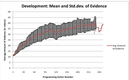
Figure 15 shows the average amount of evidence (in tokens) as a function of progress
through a tutoring session (Note: the figures presented in the body of this work stretch each
session to align their start and end. Matching figures that do not time scale the student actions
are presented in Appendix A. The time-scaled figures are easier to understand and discuss
and do not vary substantively from the figures in Appendix A). As expected, on average the
amount of evidence grew almost monotonically throughout the session. The variance in the
amount of evidence grew in the body of the session as the students got into the problem and
31 probably a result of the tutors wrapping up the session with some variance remaining due to
the different solutions.
Figure 15. Time-scaled Development Data: Mean and standard deviation of evidence.
Figure 16 compares the minimum edit and DCBN-based systems’ fraction of
evidence explained throughout a tutoring session. Both systems behaved as expected. The
minimum edit distance approach accounted for each token as quickly as it could, while the
DCBN system had to wait until sufficient evidence accumulated before it could instantiate a
higher level hypothesis and have the student’s tokens incorporated into the top-level
hypothesis. The double dip nature of the DCBN curve matched the usual session’s
32 Figure 16. Time-scaled Development Data: Comparison of minimum edit and DCBN by fraction of
evidence explained.
The dip in the DCBN’s fraction of evidence explained at the end of the session was a
result of two outlier sessions. Figure 17 shows that the majority of the sessions followed the
average path but there were two sessions that lost traction on the problem right at the end.
Note that the lower fraction of evidence explained does not mean that the evidence was not
explained somewhere in the Bayes net; it merely means that the evidence and its parent
33 Figure 17. Time-scaled Development Data: Fraction of evidence explained for all DCBN sessions.
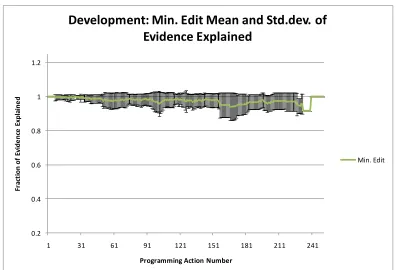
Figure 18 and Figure 19 show the mean and standard deviation of the evidence
explained fraction for the minimum edit distance and DCBN systems (providing more detail
than in Figure 16).
As can be seen in Figure 18, the minimum edit distance method behaved as expected.
It had a somewhat constant mean and standard deviation (compared to the DCBN) and
converged to the correct answer at the end of the session. The variance decreased a bit at the
34 Figure 18. Time-scaled Development Data: Minimum edit distance mean and standard deviation of
evidence explained fraction.
In Figure 19 it can be seen that the DCBN system also behaved as expected and
converged to the correct answer by session end. The variance grew substantially as the
students got into the body of the problem and (ignoring the effect of the outliers) it tapered
35 Figure 19. Time-scaled Development Data: DCBN mean and standard deviation of evidence explained
fraction.
Figure 20 shows the number of Bayes net nodes both before and after pruning. The
pruning process behaved as expected, with fewer nodes existing after the pruning step and
both curves increasing with the amount of evidence. The pre-pruning curve had a .986
correlation with the amount of evidence (Figure 15), while the post-pruning curve had a .996
correlation. This behavior matches Alvarado’s results, although SketchREAD had
36 Figure 20. Time-scaled Development Data: Number of Bayes net nodes before and after pruning.
Figure 21 shows that the variance in the pre-pruned number of nodes is very high.
This is a result of different student actions incurring different numbers of generated
hypotheses. Figure 22 shows that the number of post-pruned Bayes net nodes is far more
37 Figure 21. Time-scaled Development Data: Mean and standard deviation of pre-prune number of Bayes
net nodes.
38 Besides the number of nodes, the interconnectedness of the Bayes net is another
metric for its complexity. Figure 23 shows the average maximum number of parents in the
Bayes net both before and after pruning. As expected, the pruning reduced the
interconnectedness of the Bayes net in addition to shrinking its size. The average maximum
number of parents did increase slightly within the body of the session as more hypotheses
competed to explain the observed data.
Figure 23. Time-scaled Development Data: Pre- vs. Post-pruning maximum number of parents.
Figure 24 shows the mean and standard deviation for the pre-pruning maximum
number of parents. The maximum number of parents was highly variable due to the wide
39 deviation for the post-pruning maximum number of parents. The pruning process greatly
reduced the variability in the interconnectedness of the Bayes net.
Figure 24. Time-scaled Development Data: Mean and standard deviation of pre-pruning maximum number of parents.
Finally, Figure 26 shows the mean and maximum of the per student input character
running time. The overall mean was .37s, while the overall standard deviation was 6.11. The
variability in the execution time was driven by the pre-pruned Bayes net size and maximum
number of parents. This extreme variability makes it difficult to incorporate DCBN-based
code understanding into an ITS. These timings results were faster than those reported by
40 Figure 25. Time-scaled Development Data: Mean and standard deviation of post-pruning maximum
number of parents.
41
Test set results. The test set consisted of 10 sessions not seen during development.
The DCBN system was able to process 9 of the sessions but failed on one because of
runaway combinatorial hypothesis generation. Omitting the failed session, the DCBN system
failed to match the top-down recursive descent parser’s abstract syntax tree in five cases out
of the 155 times the student code was compileable (yielding a failure rate of 3.2%). This
matching failure never occurred at the session’s end so the DCBN was able to get back on
track.
The minimum edit distance method failed to find an answer that explained all the data
by session’s end twice. In the first case only one token was unexplained (a ―<=‖ instead of a
―<‖ in a ―for‖ loop). In the second case, 12 tokens were left unaccounted for. Creating the
missing answer would require only a minor modification to an existing answer —which the
minimum edit algorithm did correctly identify (i.e., the minimum edit system matched the
semantically closest of the five available patterns). The session on which the minimum edit
system failed was also the one on which the DCBN system diverged.
Figure 27 shows the average amount of evidence in the test set. Taking into account
noise due to the smaller sample size, it closely matches the development set (Figure 15).
(Note: all of the test set figures omit the failed session—it is treated separately later). Figure
28 compares the minimum edit and DCBN fraction of evidence throughout the session.
These results also closely match the development set’s results (Figure 16). Figure 29 shows
all of the DCBN fraction of evidence paths throughout the session. The test set had fewer
outliers than the development set. Figure 30 and Figure 31 show the mean and standard
42 reveal that in both cases the variance was greater for the test set due to unseen student
sessions (and smaller sample size).
43 Figure 28. Time-scaled Test Data: Comparison of minimum edit and DCBN by fraction of evidence
explained.
44 Figure 30. Time-scaled Test Data: Minimum edit distance mean and standard deviation of evidence
explained fraction.
45 Figure 32 through Figure 34 show the relation between the pre-pruning and
post-pruning number of Bayes net nodes. The test set had a slightly greater variability than the
development set, particularly in the pre-pruning number of nodes. The pre-pruning curve had
a correlation of .968 with the evidence curve (down from .986 in the development set), while
the post-pruning curve had a correlation of .995 (matching the development set’s .996).
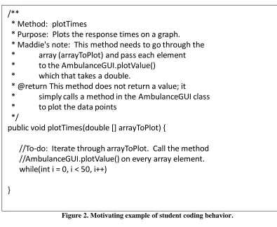
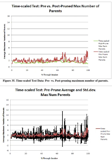
Similarly, the pre-pruning and post-pruning maximum number of parents (Figure 35 through
Figure 37) matched the development set curves but with greater variability (particularly in
the pre-pruning numbers).
46 Figure 33. Time-scaled Test Data: Mean and standard deviation of pre-prune number of Bayes net nodes.
47 Figure 35. Time-scaled Test Data: Pre- vs. Post-pruning maximum number of parents.
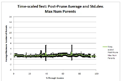
48 Figure 37. Time-scaled Test Data: Mean and standard deviation of post-pruning maximum number of
parents.
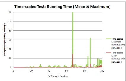
Figure 38 shows the average and maximum running time through a student session
for the test set. The mean was .53s with a standard deviation of 7.3. The test set’s times were
more variable than the development set’s (Figure 26). This is consistent with the greater
49 Figure 38. Time-scaled Test Data: Mean and maximum of running time per student character stroke.
Failed Session. The DCBN-based code understanding system failed to complete on
one of the test sessions. It ran out of memory within the SMILE library (SMILE) 65% of the
way through a session attempting to convert the causal strengths to a CPT. One limitation of
SMILE is that it does not fully exploit Noisy OR nodes and converts them to regular CPTs
prior to inference. The exponential growth of the CPT with the number of parents resulted in
SMILE attempting to allocate a 1GB block of memory.
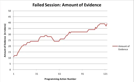
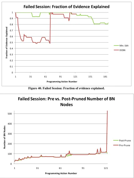
Figure 39 shows that the amount of evidence provided by the student was not
unusual. Figure 40 also reveals that the DCBN system was behaving as usual with regard to
the amount evidence for which it could account, showing the normal lag for the ―for‖ loop.
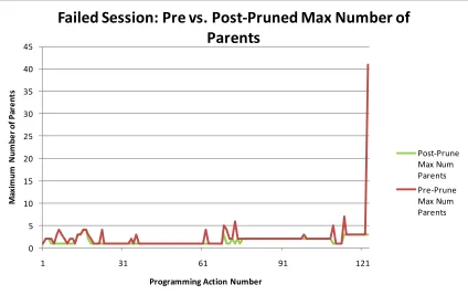
Figure 41 and Figure 42 however show that on the 123rd student action both the size of the
50 DCBN system got trapped in the combinatorial explosion of trying to reorganize statements
into blocks.
Note in Figure 40 that the minimum edit solution was also not able to deal with this
student’s solution. The minimum edit system was not able to explain the entirety of the
solution and did not converge to 1.0 at session end. The minimum edit system did, however,
select the answer key that was semantically closest to the student’s solution (i.e., the
student’s solution was a minor variation of the selected answer).
0 5 10 15 20 25 30 35 40 45 50
1 31 61 91 121
A m oun t of E vi de nc e ( in tok e ns )
Programming Action Number
Failed Session: Amount of Evidence
Amount of Evidence
51 0 0.1 0.2 0.3 0.4 0.5 0.6 0.7 0.8 0.9 1
1 31 61 91 121 151 181
Fr ac ti o n o f Ev id e n ce E xp la in e d
Programming Action Number
Failed Session: Fraction of Evidence Explained
Min. Edit DCBN
Figure 40. Failed Session: Fraction of evidence explained.
0 100 200 300 400 500
1 31 61 91 121
N um be r of B N N ode s
Programming Action Number
Failed Session: Pre vs. Post-Pruned Number of BN
Nodes
Post-Prune
Pre-Prune
52 0 5 10 15 20 25 30 35 40 45
1 31 61 91 121
M axi m um N um be r of P ar e nt s
Programming Action Number
Failed Session: Pre vs. Post-Pruned Max Number of
Parents
Post-Prune Max Num Parents Pre-Prune Max Num ParentsFigure 42. Failed Session: Pre- vs. Post-Pruned maximum Number of Parents.
Development Time. The core Bayes net construction portion of the DCBN system
took substantially greater than 30 man days to implement and debug. In contrast, it took only
1 man day to implement the minimum edit distance system and create the five answer
patterns required for the development set. The core DCBN system consists of 7962 lines of
code (omitting comments and blank lines), while the minimum edit distance system only
requires 319 lines of code (25x less). The minimum edit distance system is clearly a far
simpler system.
Qualitative. In general, the Bayes net generation and inference system behaved as expected. The Bayes net nicely handled ambiguity in the student’s code by creating multiple
counter-53 intuitive, but usually worked appropriately. In some cases, however, the Bayes net hypothesis
generation lagged far behind what a human tutor would know (i.e., a human tutor would
know the student was trying for a ―for‖ loop quite early in the ―while(i = 0, i < 50, i++)‖
example, but the DCBN would have to wait for extra evidence to formulate such a
hypothesis). This would be a potential problem for an ITS attempting to exactly emulate a
human tutor by delaying mitigation until later than a human could do so. Overall, however,
the hypothesis creation yielded a conceptually pleasing progression.
Although the quantitative analysis captures some aspects of the DCBN and minimum
edit distance performance, it is not entirely accurate. While the minimum edit solution
appears to uniformly account for student actions, it is blindly matching tokens without
considering their intent. Some of this intent is ―compiled‖ into the answers (i.e., the
minimum edit system cannot go too far astray since it has to cleave closely to the structure of
the provided answers), but the ―intelligence‖ behind the minimum edit matching is minimal
(also ―precompiled‖ into the answers). The DCBN system, at least, uses structured
knowledge of the domain to better account for student actions.
Since the actual knowledge of the student intent is ―compiled‖ into the minimum edit
answers, it is difficult to operationalize it to drive a student model. In the cases where the
minimum edit answers are compileable, an abstract syntax tree could be built for each answer
and, as tokens are matched, the explained abstract syntax tree nodes could update a student
model. This approach, however, would be difficult to extend to higher-level PROUST-like
plans and goals. DCBNs, on the other hand, could clearly be extended to support such
54 competing hypotheses with the most likely explanation updating the student model. Thus,
while minimum edit could be enhanced to support a fine grained student model, the DCBN
55
CHAPTER 4 Related Work
This work rests at the intersection of several active research areas. Prior programming
ITSs provide other sample points in the code understanding system design space. Program
understanding directly speaks to some of the requirements of the code understanding system.
Plan recognition, and particularly DCBN-based plan recognition, provides the inspiration for
the proposed approach. DCBNs are a form of knowledge-based model construction and rely
on the field of graphical models. Finally, code understanding is closely related to parsing and
compilation and relies on much of the framework and tools of that discipline.
ITSs for Programming
LISP tutor. LISP Tutor was an early cognitive tutor (Anderson & Reiser, 1985; Corbett, Anderson, and Patterson, 1988) based on Anderson’s ACT* theory of learning and
cognition. LISP Tutor’s programming knowledge was encoded as a set of about one thousand
if-then productions. Given a problem description, LISP Tutor used planning to determine a
set of acceptable solutions. Early versions of the system then monitored student actions and
immediately corrected them if they deviated from an acceptable path, using ―buggy‖
productions to both detect the bad action and drive the correction. Later versions of the
system precompiled the acceptable solutions and allowed the student to buffer their actions
for evaluation (granting greater input flexibility).
Despite its generality, LISP Tutor was actually quite restrictive. By employing a
56 student errors, initial versions of LISP Tutor greatly limited the range of student input.
Although better, later LISP Tutor versions were still very restrictive. While the student was
allowed to code ahead, the evaluation system would still proceed top to bottom
left-to-right—only characterizing the first student error and discarding ―incorrect‖ later sections.
Early LISP Tutor versions also explicitly queried the student regarding their next goal
thereby further limiting the scope of the student-action understanding problem.
LISP Tutor was evaluated through its use in a LISP mini-course and in a more
standard classroom setting. In the mini-course, students using LISP Tutor were 30% faster at
finishing the exercises and performed one standard deviation (43%) better than students
working on their own. In the standard classroom, the LISP Tutor students were 60% faster
and performed 30% better than the control students.
With regard to where it lies in the code understanding design space, LISP Tutor
greatly restricted the variability of student solutions but provided token-by-token updates.
The technology supporting LISP Tutor was complex but it was able to drive a very detailed
student model (i.e., each production could be mapped to some piece of student knowledge).
Java intelligent tutoring system. The Java Intelligent Tutoring System (JITS) (Sykes & Franek, 2003; Sykes & Franek, 2004) is a more recent tutoring system focused on
Java . JITS uses a hybrid approach to code understanding: if an answer key is provided, it
uses a simple minimum edit distance algorithm, but otherwise it uses an error-correcting
parsing approach loosely based on Aho and Peterson (1972). In the error-correcting parsing
approach, minimum edit distance is used to transform tokens into plausible inputs (i.e.,
57 then forced to add plausible tokens (e.g., generate a missing ―;‖). The changes found by the
minimum edit distance or error-correcting parsing systems are then used to drive system
interaction.
JITS represents a very different set of design decisions than LISP Tutor. The input is
very unconstrained but the student must manually press a ―parse‖ button to have JITS
evaluate their code. The technology needed for JITS is far less than that required for LISP
Tutor and correspondingly does lose some ability to model student knowledge (particularly
for the pure minimum edit distance path).
PROUST. PROUST (Johnson & Soloway, 1985; Johnson, 1986) was a planning-based program understanding/debugging system planning-based on Soloway et al.’s theory of
programming (Soloway & Ehrlich, 1984; Soloway, 1986; Spohrer & Soloway, 1985).
PROUST’s programming knowledge was encoded as a set of goals and plans which, given a
description of the problem and a compileable student solution, were used to determine a
probable student implementation path. Heuristics were used to constrain the search space to
the more probable goal-plan decompositions (e.g., goal A is usually implemented via plan B)
and to decide amongst competing alternatives (e.g., if two goal-plan decompositions explain
the same data, select the one that has the less serious error). Matching between the generated
and student code was used to evaluate the proposed paths. PROUST’s matching system could
resolve near misses (and thus account for additional variability) by altering the code via
common transformations. Problem areas in the student code were identified by the
appearance of ―buggy‖ plans in the decomposition and mismatches between the generated