ABSTRACT
SUBBIAH, SETHURAMAN. CloneScale: Distributed Resource Scaling for Virtualized Cloud Systems. (Under the direction of Dr. Xiaohui (Helen) Gu.)
Infrastructure-as-a-Service (IaaS) cloud systems often use the virtualization technology to
share resources among different users and provide isolation among uncooperative users. We can
use a resource cap to limit the resource consumption of one virtual machine (VM). However,
the resource requirements of an application are rarely static, varying with workload intensity
and mix changes. Many existing techniques use machine learning, control theory, or queuing
theory to determine the application resource demand on the fly. When the local resource cannot
satisfy a VM’s resource requirement, previous work has employed live VM migration to move
the VM to a host with sufficient resources. However, it is possible that not a single host can
satisfy the resource requirement of the resource-intensive VM. Under those circumstances, it is
desirable to perform distributed resource scaling that can aggregate the resources of multiple
hosts to serve one application.
In this thesis, we present CloneScale, a system that leverages VM cloning to dynamically
distribute the workload of one application among multiple hosts. The newly cloned VM will be
the replica of the parent VM including its memory and disk state, yet they act as two
indepen-dent VMs. VM cloning is chosen to reduce the time taken for the VM to resume processing.
CloneScale provides load balancing among all the cloned VMs with minimal application
knowl-edge. Besides resource depletion, progress rate and SLO violations can also be used to trigger
VM cloning. We have implemented a prototype of CloneScale over the Kernel-based Virtual
Machine (KVM) platform and shown that we can effectively clone an application VM and start
c
Copyright 2012 by Sethuraman Subbiah
CloneScale: Distributed Resource Scaling for Virtualized Cloud Systems
by
Sethuraman Subbiah
A thesis submitted to the Graduate Faculty of North Carolina State University
in partial fulfillment of the requirements for the Degree of
Master of Science
Computer Science
Raleigh, North Carolina
2012
APPROVED BY:
Dr. Frank Mueller Dr. Xiaosong Ma
DEDICATION
BIOGRAPHY
Sethurman Subbiah was born in a town called Salem, Tamil Nadu, India and brought up in
a huge and beautiful city called Chennai. He recieved his Bachelor of Technology in
Informa-tion Technology from Sri Venkateswara College of Engineering (Affiliated to Anna University),
Chennai, India in May 2009. With the defense of this thesis, he will recieve the Master of
Sci-ence in Computer SciSci-ence from North Carolina State University in December 2011. He intends
to start his full-time employment at NetApp Inc., Sunnyvale after graduation. His research
ACKNOWLEDGEMENTS
I would like to thank my advisor, Dr. Xiaohui (Helen) Gu for her invaluable guidance in
performing research and writing this thesis. Furthermore, I would like to thank my advisor for
giving me such a wide exposure in this field. I thank Dr. Xiaosong Ma and Dr. Frank Mueller
for their kind consent to serve on my thesis committee. I am extremely thankful to all DANCE
research group members especially to Zhiming Shen, Yongmin Tan and Hiep Nguyen for their
advice and help during my research.
I would also like to thank all my friends for their help, motivation and encouragement
during my graduate study: Arun Natarajan, Anand Parthasarathi, Dinesh Radhakrishnan,
SriKrishna Gopu, Vivek Devarajan, Sudharshan Prasad, Vijay Shanmugasundaram, Koushik
Krishnakumar, Manikandan Sivanesan and Gopinath Chandrasekaran. Finally, my deepest
gratitude goes to my father Mr. S. Subbiah, my mother Dr. S. Meenakshi, my brother S. Vijay
TABLE OF CONTENTS
List of Figures . . . vi
Chapter 1 Introduction . . . 1
Chapter 2 Background. . . 4
2.1 Multi-Tenant Cloud Systems . . . 4
2.2 CloudScale : Elastic Resource Scaling for Multi-Tenant Cloud Systems . . . 5
2.2.1 Fast under-estimation correction . . . 5
2.2.2 Online adaptive padding . . . 5
2.2.3 Scaling conflict handling . . . 6
2.2.4 Predictive frequency/voltage scaling . . . 6
2.3 Apache Hadoop Mapreduce . . . 6
2.3.1 Hadoop Architecture . . . 7
2.3.2 HDFS Architecture . . . 7
2.4 RUBiS - Rice University Bidding System . . . 8
Chapter 3 System Design . . . 9
3.1 Overview . . . 9
3.2 VM cloning . . . 11
3.2.1 Hot Cloning . . . 11
3.2.2 Cold Cloning . . . 12
3.3 VM Reconfiguration . . . 13
3.3.1 IP Reconfiguration . . . 13
3.3.2 Post-Cloning Application Reconfiguration . . . 14
3.4 Prediction-Driven Cloning . . . 15
3.4.1 Prediction . . . 15
3.4.2 Predictive cloning . . . 16
3.4.3 Predictive Down-Scaling . . . 18
Chapter 4 Experimental Evaluation . . . 19
4.1 Experimental Setup . . . 19
4.2 Prediction . . . 20
4.3 Cloning . . . 22
Chapter 5 Related Work . . . 40
Chapter 6 Conclusion and Future work . . . 46
LIST OF FIGURES
Figure 3.1 CloneScale architecture Diagram . . . 10
Figure 4.1 Comparison between the predicted and actual CPU trace . . . 21
Figure 4.2 Prediction accuracy under different lead time . . . 21
Figure 4.3 Time series of SLO violation rate for different cloning schemes . . . 24
Figure 4.4 Impact of cloning on the cloned VM and co-allocated VM . . . 25
Figure 4.5 Comparison between time taken for cold cloning and hot cloning . . . 27
Figure 4.6 Comparison of average delay after hot and cold cloning of web server and MySQL database server . . . 28
Figure 4.7 Comparison between hot and cold cloning of a web server . . . 29
Figure 4.8 Comparison between hot and cold cloning of a MySQL database server . 31 Figure 4.9 Cold cloning warmup phase for MySQL database server . . . 32
Figure 4.10 Comparison between completion rate of hadoop map node without cloning and with hot cloning . . . 34
Figure 4.11 Comparison of hot and cold cloning of a hadoop map node . . . 35
Chapter 1
Introduction
Cloud computing has emerged as a very popular technology among startups and new developers
with its pay-as-you-go model. It provides a hassle free and cost-effective solution mainly because
of cloud elasticity. Cloud elasticity provides the capability to dynamically allocate and reclaim
resource in response to the changes in workload. A particular Facebook application became
very prominent and the user base increased from 25,000 to 250,000 in three days with signing-up
20,000 new users per hour at peak [2]. As the scale of applications and their hosting environment
expands, the complexity and overhead involved in managing the cloud environment increases.
It creates the need for automating dynamic VM resource allocation.
Amazon EC2 provides an auto scaling feature [1] where new VMs can be added or removed
dynamically based on the user defined policy. For example, adding a new node when the CPU
usage exceeds above 90% and removing a node when the CPU usage goes below 10%. It takes
several minutes to start a VM from the base image, followed by the time taken to set up the
environment and start the application. Since the VM is freshly booted, the application will
require a warm up time to populate the cache. All together, the time taken for the new VM to
work at its maximum efficiency is in minutes. Moreover, the user is burdened with the process
of setting up the environment, starting the application, and deciding the scaling policy.
signifi-cantly reduce the time taken for the new VM to start servicing requests at its peak efficiency.
We also support prediction-driven cloning, where the cloning operation can be started before
the VM resource demands increase beyond the resource available on that host. This helps to
reduce the application’s SLO violation time. Our system is intended to perform with least
human intervention and minimal application knowledge.
To design such a system, we need to address three challenges: i) performing efficient cloning,
ii) making the application inside the VM compatible with cloning, and iii) when to perform
cloning.
In order to perform efficient cloning, we present two variations of cloning mechanisms,
namely hot cloning and cold cloning. In hot cloning, we stop the parent VM temporarily, save
all its memory content to a state file, and use this state file to create a clone. Hot cloning can
propagate the memory state of the parent VM to the cloned VM. In cold cloning, we create
a new cloned VM from an existing template. This template is created before the application
starts processing any requests. Cold cloning can be used for applications whose memory and
disk state do not change a lot during runtime. The decision on which cloning mechanism to
use is made dynamically during runtime.
To make the application compatible with cloning, we present a generic user interface. The
application user is expected to provide minimal information about the application running inside
the VM and a script to re-configure the application after cloning. In order to decide when to
trigger cloning, we present a scaling policy for the user. We use a prediction model for every VM
to predict the future resource demands of that particular VM. When the predicted resource
demand exceeds the residual resources available on that host, we trigger cloning. Stateless
application does not suffer any loss of information when a node is terminated. Thus, when
we predict the resource usage of a VM running stateless application to go below a minimum
threshold, we terminate the unnecessary VM.
We have implemented a prototype of CloneScale on top of the Kernel-based Virtual Machine
hot cloning with full state propagation in tens of seconds. We have evaluated our work against
Chapter 2
Background
In this chapter, we introduce the background for the CloneScale work. Our current work aims
at dynamically distributing the workload of one application among multiple nodes using VM
cloning and load balancing techniques. Hadoop MapReduce and RUBiS are the two real world
applications we use to evaluate our work. This chapter aims at providing good background
knowledge on these important topics.
2.1
Multi-Tenant Cloud Systems
The pay-as-you-go model has been the driving force of cloud computing. Cloud users, called
tenants, can lease computing resources and pay only for what they use. Multi-tenant cloud
systems let multiple users share one common cloud infrastructure, and also provide various
features such as automatic scale-up and scale-down, and resource isolation among co-allocated
users. Multi-tenant cloud systems are appropriate for startups and new developers to kick start
their applications by providing a more cost-effective solution than buying physical computing
2.2
CloudScale :
Elastic Resource Scaling for Multi-Tenant
Cloud Systems
CloudScale performs prediction driven resource scaling in a multi-tenant cloud system. In order
to provide performance isolation, CloudScale aims at setting a suitable resource cap for VMs.
A low cap may lead to SLO violations and a generous cap may lead to wastage of resources.
Thus, Cloudscale monitors the resource usage of a domain, use prediction algorithms to predict
the future resource usage and set a suitable cap.
2.2.1 Fast under-estimation correction
Achieving 100 percent prediction accuracy is hardly possible. If the predicted CPU value is lower
than the real demand, the newly set CPU cap will not be sufficient for the application. Under
provisioning causes undesirable performance impact. Under provisioning is detected by the
resource pressure metric or SLO feedback from the application. However, the exact requirement
is unknown because the application cannot consume more resource than the resource cap. To
address this problem, CloudScale raises the resource cap exponentially until it overcomes under
provisioning.
2.2.2 Online adaptive padding
To avoid underestimation errors, CloudScale provides a mechanism called proactive padding
scheme. Based on our observations, the underestimation errors are often caused by bursts in
workload.
CloudScale employs burst based padding to accommodate bursts. The burst pattern is
extracted using signal-processing techniques such as FFT (Fast Fourier Transform). The
fre-quency of burst appearance (burst density) is calculated from the burst pattern. The padding
value is calculated based on the burst density.
Cloud-Scale calculates the padding value based on the degree of deviation of recent predictions from
the actual resource usage values. A sufficient padding will ensure less under prediction in the
future and also provides enough resources.
2.2.3 Scaling conflict handling
In a multi-tenant cloud system, a host may contain multiple VMs. Each VM will try to scale
up or down based on the predicted value. Thus, it is normal to encounter a scaling conflict
when the total resource demand exceeds the capacity. CloudScale aims at handling scaling
conflicts among co-allocated applications with minimal SLO impact. Long-term prediction
lends a helping hand in predicting the conflict early. A conflict prediction model is built to find
out the time of occurrence, intensity, and duration of conflict. A suitable solution is achieved
by comparing the SLO penalties of ignoring a few scale-up requirements by applications with
migrating VMs out of the box.
2.2.4 Predictive frequency/voltage scaling
Cloudscale couples VM CPU scaling and dynamic voltage and frequency scaling (DVFS) to
convert unused resources into energy savings. For example, if the resource demand prediction
model predicts the total CPU usage of the host as 50%, we can half the operational frequency
and double the caps of all VMs. Thus, we slow down the CPU to save energy without affecting
the application SLO.
2.3
Apache Hadoop Mapreduce
MapReduce is a programing paradigm used for processing huge amount of data in parallel.
Apache Hadoop is a MapReduce implementation in Java, heavily used in real world by Yahoo,
Facebook etc. A MapReduce program consists of two phases called Map phase and Reduce
phase. The input data is divided into chunks for processing by map tasks. The Map function
interme-diate results are produced, a split function (essentially a hash function) partitions the records
into disjoint buckets by applying the hash function to the keys of the records. These map
buckets are then written to the local disk. A number of map instances would be running on a
computing cluster. The second phase is known as the Reduce phase. Records with the same
hash value are sent to the same reducer. Each reducer processes the record assigned to it and
writes the record to the output file. For example, Wordcount is one of the Hadoop applications
we use. It counts the number of appearances of each word in a collection of text files.
2.3.1 Hadoop Architecture
Hadoop framework follows master/slave architecture. The master node consists of jobtracker
and namenode. The jobs are submitted to the jobtracker. The jobtracker manages the
sub-mitted jobs and schedules map and reduce tasks with the knowledge of the data location. The
tasktrackers at the slaves perform the computation.
2.3.2 HDFS Architecture
Hadoop distributed file system is a distributed file system designed based on the Google File
System. The features of HDFS include storing huge amount of data, providing reliability and
scalability.
The master holds the namenode, which maintains metadata of the entire filesystem.
Na-menode performs the bookkeeping while the original information is stored in datanodes. HDFS
provides fault tolerance through data replication. The user can configure the replication factor.
Different data nodes host the replicas. There can be only one master node at any instant.
Thus, master will be a single point of failure. Since the participation of namenode is less, the
2.4
RUBiS - Rice University Bidding System
We use RUBiS as an auction-site benchmarking tool. This benchmark helps us validate ourselves
with the real-world workloads. Several versions of RUBiS are implemented including PHP, Java
servlets and EJB version. Our experiments make use of the PHP version. The PHP version
consists of an Apache Webserver and a backend MySQL Database server. The client will be
able to establish a separate HTTP connection at the beginning of a session and close it at the
end. The client can perform various functionalities such as browse items, bid for items, buy
items and sell items. RUBiS provides two types of workloads: browsing, and bidding mix. The
browsing mix only includes read only interactions. In contrast, the bidding mix provides both
Chapter 3
System Design
In this chapter we present the overview of our approach, and then we introduce the two VM
cloning techniques, followed by the generic user interface that we provide to configure the
application after cloning, and finally we will provide information about the CloneScale policies.
3.1
Overview
CloneScale has two important components, the CloneScale master and CloneScale slave, and
is built on top of the KVM hypervisor. The CloneScale slave resides within each host in the
cloud system, providing VM manipulation and monitoring functions. The CloneScale master
has a global view of the entire system and performs cloning based on requests from CloneScale
slaves. Figure 3.1 shows the overall architecture of the CloneScale system.
CloneScale slave uses a monitoring tool based on libvirt to monitor the guest VMs resource
usage from the host OS. The monitored metrics include CPU consumption, memory allocated,
network traffic and disk I/O statistics. The resource usage time series are fed into an online
resource demand prediction model that uses a hybrid prediction model to predict the future
resource demands. Prediction helps us foresee the resource requirement and trigger cloning if
necessary.
Host n Host 2
Host 1
VM + Application
Application Reconfiguration
Module
Linux + KVM
CloneScale Slave Resource Monitor Prediction Module Clone Scale Policy CloneScale Master Cloning Module Clone Co-ordinator Resource usage time Series Predicted resource demands Clonning Request Cloning decision Perform Cloning
Figure 3.1: CloneScale architecture Diagram
than the resource available on the host. The CloneScale master then creates a clone on the
next available free host. By doing so, the application will be distributed among different hosts,
enabling additional capacity to handle the anticipated load increase. After cloning, CloneScale
modifies the newly cloned VM and performs some application specific changes to seamlessly
scale the application.
Stateful applications cannot be arbitrarily terminated, while stateless applications will not
suffer any loss of information. Thus, with additional information that the application is
state-less, we can provide a much more efficient solution. When the predicted resource demands are
less than the minimum threshold, we can turn off unnecessary VMs.
3.2
VM cloning
CloneScale is a system that leverages VM cloning to dynamically distribute the workload of one
application among multiple hosts with minimal SLO impact. In order to make cloning more
efficient, we provide two variants of cloning in this thesis: hot cloning and cold cloning.
3.2.1 Hot Cloning
To initiate cloning, the CloneScale slave sends a message to the CloneScale master, containing
the keyword “clone request”, the target VM’s domain name and IP address and the host IP. On
receiving a cloning request, the CloneScale master stops the VM temporarily and transfers its
memory contents to an external state file using the Virsh save command. Virsh is a management
user interface based on libvirt that can be used to create, pause, save, restore, list, and shutdown
domains. To extract the VM’s disk state, CloneScale leverages the QEMU Copy On Write
(QCOW2) image format feature to create an incremental QCOW2 image based on the parent
VM’s disk image. QCOW2 is the native image format of QEMU, and creating an instantaneous
incremental copy-on-write image is the major advantage of qcow2 image format. After creating
an incremental copy, QEMU will treat the base image as read-only, and will store all new writes
to the incremental QCOW2 image. Since the base image is changed to read-only format, it
cannot be further used to serve the parent VM. Thus while cloning, we create two incremental
QCOW2 images from the base image to restore the parent and the cloned VM. The incremental
images should always be linked with the base image, and therefore they must remain together
on a shared storage. For this purpose, we store all our images in a network-attached storage
(NAS). We can create an incremental image over an incremental image, but doing so in this
recursive manner will deteriorate the performance of the VM.
The CloneScale master restores the parent VM from the memory state file and an
incre-mental QCOW2 disk image using the Virsh restore interface. However, the Virsh save interface
saves the configuration xml inside the memory state file. The xml configuration in the state file
incremental disk image, we have to modify the xml configuration. The master uses the Virsh
save-image-dumpxml to obtain the xml saved in the memory state file header. The master
modifies the xml and restores the parent VM using the memory-state file and the modified xml.
The next available free host is chosen to host the newly cloned VM. Since the real requirement
is unknown, it is safe to choose a free host. The xml configuration file is modified to point
to a new incremental disk image. The cloned VM is restored with the memory-state file and
the modified xml file using the Virsh restore interface. The main advantage of hot cloning is
the copying of state from the parent VM to cloned VM. This avoids the initial warm-up time
required for the cloned VM to start performing at its peak efficiency.
3.2.2 Cold Cloning
In cold cloning, a new VM is cloned from a VM template instead of a running VM. We perform
cold cloning for VM hosting applications whose state can be determined in advance. The VM
template consists of a QCOW2 base image and an existing state file. CloneScale master creates
this template when the application was deployed in the cloud for the first time. The template
is created in a process similar to hot cloning mentioned in section 3.2.1 but this template is
created before the application starts processing any requests and it is stored in NAS. Thus,
we can neglect this downtime observed when calculating the efficiency of this mechanism, as it
does not affect the application’s SLO. To initiate cloning, the CloneScale slave sends a cloning
request as we mentioned in section 3.2.1. The CloneScale master responds to this cloning
request by choosing a suitable host and deploys a new VM at that host. To deploy a new VM,
we make an incremental QCOW2 image from the base image in the VM template and use the
Virsh restore interface to start a new VM with the help of the newly created incremental disk
image and exiting VM state image. Since we are creating the VM with the state of the OS
and the application before processing any requests, the newly created clone will only hold a
minimal state. However, on the other hand, the new VM can be created in a very short period
3.3
VM Reconfiguration
3.3.1 IP Reconfiguration
Since the newly cloned VM will be the exact copy of the parent VM, it will hold the same IP
address as its parent. Once the cloned VM is restored, a startup script performs the following
actions in sequence: i) Disable the VM network using IPtables, ii) Mount the cd in the standard
mount point /cd, iii) Execute the network configuration script available inside the cd, and iv)
Enable the VM network using IPtables.
To make sure this startup script is executed immediately after the VM restore, we SSH into
the VM and execute this startup script before initiating the cloning process. The startup script
has a small sleep period (five seconds in our experiments) before configuring the network. This
sleep period is to ensure that the network configuration starts after the VM cloning. We have to
note that the startup script will be executed in both the parent and cloned VMs, but we ensure
that no network changes are made in the parent by comparing the VM’s hostname with the
hostname provided through the cd and configuring the network only when they are different.
When the memory state was saved, there may be some on-going processes that may try to
communicate to a different machine with the old IP, which may cause some inconsistencies. For
this reason, we disable the network before the cloned VM gets a new IP address.
After restoring the cloned VM, the master has to pass a new MAC address into the VM.
However, the cloned VM cannot be accessed using the network. Hence, we created a virtual CD
ISO file containing the new mac address and hostname along with the network configuration
script and application post-configuration script. The virtual cd is added using the VM
config-uration xml before the cloned VM is restored. The network configconfig-uration script changes the
VM’s mac address internally, restarts the network service to obtain a new IP address using the
DHCP protocol and triggers the application post-configuration script. The functionality of the
network configuration script can be included within the startup script but following this
the network. An example to support this statement is available in the forthcoming section.
3.3.2 Post-Cloning Application Reconfiguration
After attaining a new IP address, the cloned VM is available to use. However, the application
running inside the VM will continue processing the requests that were started before cloning.
Since we clone a running VM, it is natural to expect the application to be processing requests
before cloning initiation. We provide a user interface which can be used to specify the required
information regarding the application. We provide a generalized user interface in the form of
an xml file. This xml file poses the following questions to the user: i) Can we clone this VM?,
ii) Is this a stateless application?, iii) What type of application is this?, iv) What is the path to
post-configuration script?, v) Approximate time taken for application reconfiguration, vi) Does
the application have its own load balancer?, vii) Which port has to be load balanced? and viii)
What will be the type of incoming requests to the load balancer ?
As soon as a new VM is created, CloneScale slave parses this XML file and populates the VM
settings file and creates one file per tier. The CloneScale master reads this file before performing
a cloning operation. The VM settings file will hold information that aids the master in deciding
whether cloning is viable, if yes, what type of cloning should be performed on that VM (hot
or cold). There are few applications that cannot be cloned, for example, we cannot clone a
hadoop master node. There can be only one master node in a Hadoop cluster. CloneScale also
provides a haproxy load balancer to every application. The user to work with his application can
configure this load balancer at the beginning. Besides the xml, we also require an application
post cloning configuration script. The application post cloning configuration script provided
by the user is expected to handle requests that were started by the parent VM before cloning,
making changes to the application which has modules that are bound to the host-name or IP
address of the VM and adding the cloned VM’s IP to the load balancer.
To the best of our knowledge, the most commonly used cloud applications such as web
balanced by adding the cloned VM’s IP to the load balancer for balancing a specific incoming
port, for example port 80 for apache web server and port 3306 for MySql database server. For
certain applications like Hadoop, it has its own load balancer called the job tracker. In Hadoop,
the VM hostname is considered as a unique identifier, thus the previously running task tracker
and data node processes will hold the host name of its parent. These processes has to be
stopped before the VM gets a new IP and host name, followed by starting the task tracker and
datanode with the new hostname. Once the task tracker is started, it automatically contacts
the job tracker and adds itself to the existing cluster. As mentioned in section 3.3.1, having a
network configuration script separated from the startup script gives us the flexibility to execute
the post-configuration script before or after obtaining a new IP address and host name. At
present, we have proved our CloneScale can work successfully with apache web server, MySQL
database server and apache Hadoop. The MySQL database that we use in our experiments
only caters read-only requests. Database writes and other workload patterns or applications
that alters the state of the application is not supported by CloneScale at present.
3.4
Prediction-Driven Cloning
3.4.1 Prediction
During VM cloning, the VM is stopped to transfer the VM memory, register values and cache
to a state file. The parent VM we are trying to clone has a downtime. Thus, VM cloning is not
a very cheap process. Using a reactive approach will trigger cloning when the VM is already
under provisioned. This will lead to huge SLO violations. CloneScale uses resource prediction
algorithm to proactively trigger cloning before the VM resource demands exceed the residual
resource on the host.
CloneScale uses two complementary resource prediction techniques, signatudriven
re-source prediction and state-driven rere-source prediction to trigger cloning. Initially, the
model uses the signature to predict the future resource requirement. Otherwise, the prediction
model uses discrete-time Markov chain to predict the future resource demands.
CloneScale slave resides on the host OS and monitors the resource usage of the guest VMs.
At present, CloneScale mostly performs scaling based on CPU usage. The metric used for
prediction should directly correlate to the measure of client’s service level objective (e.g. average
delay) and we believe CPU usage is one such metric. CloneScale can also use different metrics
based on the application needs such as application progress rate for Hadoop. The length of the
time we wish to predict is the sum of the time taken for cloning a VM and time taken for the
cloned VM to continue processing requests. This represents the time between clone initiations
and when the new VM will be useful. The training window sizetw differs between experiments,
but mostly we use a training window size between 100 and 2000 seconds. Later, the model is
retrained every eight seconds usingtw recent samples and a new prediction is made every eight
seconds. The time taken to clone a VM depends upon the memory size of the VM and does
not show much variation. We have already calculated the average time taken for hot and cold
cloning of VMs with different memory size. We use this average cloning time to define our look
ahead window size or how far we need to look into the future, which helps us clone the VM
before it gets overloaded.
3.4.2 Predictive cloning
CloneScale slave employs resource monitoring and prediction to foresee the resource demands
of a VM. We use prediction to trigger cloning before the system is underprovisioned. The look
ahead window dictates how long we would like to predict the future. The duration of a
look-ahead window is set as twice the time taken for cloning a VM. The first half of the look look-ahead
window denotes the cloning period and the second half of the look ahead window denotes the
period after cloning. Thus, we will be able to observe the system’s resource demand after the
cloning period and decide whether the newly cloned VM will aid in reducing the SLO
threshold, CloneScale slave triggers cloning. This maximum threshold is a configurable
param-eter, it can be configured based on the SLO needs. Setting a very high threshold gives very less
importance to SLO and effectively reduces the number of clone requests. On the other hand,
setting a very low threshold will trigger cloning too often, which will affect the application SLO
and also overprovisions resources. Thus, it is really important to choose the right threshold.
Once the cloning is triggered, the CloneScale master choses the next available free host as
the cloning destination and parses the settings file corresponding to the domain name. The
user’s information regarding the application is retrieved by the CloneScale slave and it creates
a settings file which helps the CloneScale master to identify whether: 1) the VM can be cloned,
2) which cloning mechanism should be used (hot or cold), 3) What is the application type? 4) Is
the VM using our load balancer?, 5) which port has to be load balanced. Since CloneScale slaves
reside on all hosts and are independent, there can be multiple scaling requests to the master.
The master should accept only one scaling request from a tier and ignore rest of the requests.
For example, let there be three webservers servicing requests. When the workload gets highly
intensive such that the three webservers will not be enough to satisfy all requests. In this case,
the CloneScale slaves running in the host OS will predict the total resource available on that
host is insufficient. All three hosts will trigger cloning. In this case, CloneScale master creates
just one clone based on the first received request and sends a message to the load balancer
to distribute load to the newly created clone. If four servers cannot handle the request again
another clone will be initiated. Creating a clone for each request will stop all three running
VMs simultaneously, which will make the application SLO suffer more.
Immediately after the parent VM is restored, it will experience few early spikes till the newly
cloned VM starts servicing requests. These spikes may invoke another cloning operation, which
is a false call but it stops the parent VM once again to save the memory state and create a new
clone leading to further SLO violations. Thus after the completion of a cloning operation, we
ip address, sleep time in the startup script and the approximate application reconfiguration
time. Any further cloning requests from the same tier during that locked period is ignored.
3.4.3 Predictive Down-Scaling
For stateless applications, besides cold cloning, CloneScale also performs distributed down-scale.
When more than 3/4th (a heuristic value) of the look-ahead window is below the minimum threshold, then down scaling is triggered. During down-scaling, IP address of the first VM to
trigger cloning is removed from the list of load sharing nodes at the load balancer. However, the
VM is not immediately turned off. We keep the VM at a standby state for a time period ofts
seconds. ts refers to the time taken to perform cold cloning. Any further scale up requirements
within the nexttsseconds can be satisfied immediately by informing the load balancer to include
Chapter 4
Experimental Evaluation
In this chapter we discuss various results we collected using our system.
4.1
Experimental Setup
The experiments were conducted on the Hybrid Green Cloud Computing (HGCC) Cluster at
North Carolina State University. Each HGCC node has an Intel Xeon 3440 2.56 Ghz quad-core
processor, 250 GB hard disk, 8GB Memory, 1Gbps network bandwidth, and runs CentOS 6.0
64 bit with QEMU-KVM 0.12.1. The HGCC cluster has a network-attached storage (NAS)
with size 6TB in RAID5 storage technology. 2 TB of our NAS is used for parity. All images are
maintained on the NAS and we leverage this advantage to create incremental QCOW2 images.
Our resource monitoring code was written based on libvirt 0.9.4 library. We use the virsh
management interface to create, stop, save, and restore guest VMs. The CloneScale master
runs on a single node (HGCC13 in our cluster), which has the same configuration as mentioned
above. The master has a global view of the entire system and performs cloning and down-scaling
on behalf of CloneScale slaves.
The guest VMs are usually configured with 1 VCPU core and 1 GB memory. Each guest
VM runs Centos 5.2 64 bit and is connected to the network using the bridge interface ”br0” in
CPU, memory, disk and network IO. The resource metrics are collected at different sampling
rates based on the type of cloning technique used (hot or cold cloning) and we currently perform
scaling based on the CPU metric alone. We used two different kinds of workloads to evaluate
our work, the RUBiS and Hadoop. Section 2.2 and 2.3 gives a brief overview about both
applications. In RUBiS, we let the workload generator to track the response time of the HTTP
requests it made. The SLO violation rate is the fraction of requests that has response time
greater than the pre-defined SLO threshold during each experiment. The SLO threshold varies
in our experiments based on the intensity of the workload used. In Hadoop, we are using the
word count on 282 text files as a workload to evaluate our system.
4.2
Prediction
During cloning, the VM will be temporarily suspended and the memory will be transferred to
a state file. This action takes tens of seconds and performing this action during peak usage
will provide unacceptable results. Thus, we try to use a prediction algorithm to predict the
future resource usage of the VM and perform cloning when the VM’s CPU usage is predicted
to exceed the maximum threshold. Figure 4.1 shows a sample real and predicted trace.
To measure the accuracy of our long term prediction algorithm, we collected a six hour CPU
trace of a RUBiS webserver and used this trace to test our prediction model. We feed this CPU
trace as input to our prediction algorithm to get a list of predictions. We had a fixed training
window of 100 samples and varied the sampling interval between one second and ten seconds.
We retrain the model every eight seconds and predict the next eight steps. We mark all the
time instances where cloning has to be triggered, then use our prediction algorithm to predict
when cloning has to be triggered with different look ahead window size. From the predictions,
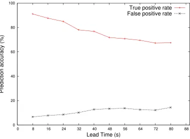
we calculate: i) Number of true positives (Ntp) - the CPU usage of the VM is predicted to
exceed the maximum threshold correctly, ii) Number of false negatives (Nf n) - the CPU usage
of the VM exceeds the maximum threshold but it is not predicted, iii) Number of false positives
0 20 40 60 80 100 120
200 300 400 500 600 700
CPU (%)
Time (s)
Actual value Predicted value
Figure 4.1: Comparison between the predicted and actual CPU trace
0 20 40 60 80 100
0 8 16 24 32 40 48 56 64 72 80 88
Prediction accuracy (%)
Lead Time (s)
True positive rate False positive rate
happen, and iv) Number of True negatives (Ntn) - the CPU usage of the VM is predicted to
stay within the maximum threshold correctly. The true positive rate Tp and the false positive
rateFp are calculated using the standard formulaTp =Ntp/(Ntp+Nf n);Fp =Nf p/(Nf p+Ntn).
Figure 4.2 shows the true positive rate and the false positive rate of our long term prediction
algorithm under different lead time window sizes. The prediction model has a true positive
rate of 91.5% for a lead time of eight seconds and reduces when the lead time window size
increases. Since cloning is not a cheap process, false alarms will cause unnecessary cloning and
unnecessary SLO penalities. Improving the prediction accuracy is one of our main future works.
4.3
Cloning
From the previous experiments, it is evident that our prediction has high true positive rates and
it can be used to drive cloning. We further investigated this issue by comparing the reactive
approach against our proactive approach to trigger cloning. We have modified the RUBiS
workload generator to send UDP message when a SLO violation is recorded. In the reactive
approach, cloning is triggered when three continuous SLO violations are reported. Whereas
in a proactive approach, we use a moving window with eight recent CPU samples and a look
ahead window containing the predicted next eight steps. Here, cloning is triggered when any
five samples in either one of the windows exceed the maximum threshold. There are a few
special scenarios where the CPU usage remains very low for a long duration and the workload
rises almost instantly (e.g. consider a situation where a university releases exam results at 6.00
PM. Every student tries to access the same website to view his/her results). In such scenarios,
if we use only the look ahead window, the model will take few minutes for catching up to the
current trend. Whereas, using both the look ahead and moving window will identify the need
for cloning immediately. We use RUBiS system with one front-end webserver and two back-end
databases to perform this experiment. The client workload generator creates 400 threads to
browse the webserver and the workload generator tracks the delay observed by each thread. We
than the pre-defined threshold per second. Using this method, we plot the SLO violation trace
with time as x-axis and the SLO violation rate as y-axis.
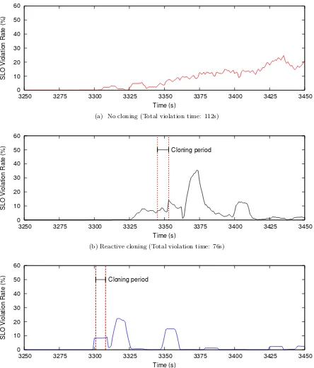
Figure 4.3a shows the violation rate observed in the absence of CloneScale. The SLO
violations start from 3330 seconds. The initial small violations observed between seconds 3310
and 3320 is due to the moving average. Since, the observed raw trace was hard to read, we
calculated the average with a moving window of size 15 to smooth the curve. The violation
observed between seconds 3310 and 3320 is due to small violation observed for two seconds.
Figure 4.3b shows the effect of using a reactive based approach. After receiving three continuous
violations, cold cloning is triggered. Since webservers are stateless, cold cloning technique is
more apt for cloning a webserver than hot cloning. The small peak observed between 3360 and
3380 is due to the moving average that we calculate. In reality, we observe only a single very
high spike for two seconds caused by the load balancer. The load balancer should be restarted
after adding a newly cloned node for the change to take effect. Since it takes few seconds for
the newly cloned VM to start servicing requests and the system has already started observing
violations, we see an impact in performance. Figure 4.3c shows the performance of CloneScale
which uses prediction driven cloning. We use a prediction model to foresee the future resource
usage and make a cloning decision based on this prediction. Thus, before the system starts
observing violations we perform cloning. This helps in reducing the violations.
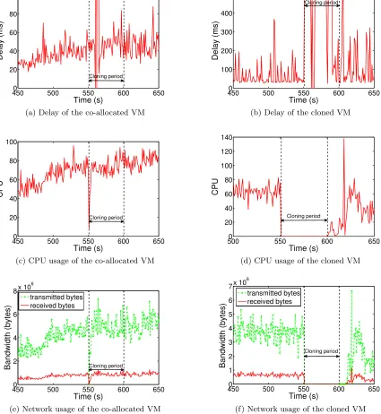
In Figure 4.4 we compare the impact of cloning on the cloned and co-allocated VMs. We
are trying to compare three different metrics among the cloned and co-allocated VM. The three
metrics we chose to compare are average delay, CPU usage and network usage of both the cloned
and co-allocated VMs. We believe these three metrics will help us understand the impact from
all three dimensions. Since we are writing the VM’s memory to a state file in NAS, we believe
network will be a very good metric to study the impact.
These experiments are performed with two VMs on a single host. Both VMs host a RUBiS
webserver belonging to different applications. We perform hot cloning and study the impact of
0 10 20 30 40 50 60
3250 3275 3300 3325 3350 3375 3400 3425 3450
SLO Violation Rate (%)
Time (s)
(a) No cloning (Total violation time: 112s)
0 10 20 30 40 50 60
3250 3275 3300 3325 3350 3375 3400 3425 3450
SLO Violation Rate (%)
Time (s)
Cloning period
(b) Reactive cloning (Total violation time: 76s)
0 10 20 30 40 50 60
3250 3275 3300 3325 3350 3375 3400 3425 3450
SLO Violation Rate (%)
Time (s) Cloning period
(c) Proactive cloning (Total violation time: 36s)
4500 500 550 600 650 20 40 60 80 100 Time (s) Delay (ms) Cloning period
(a) Delay of the co-allocated VM
4500 500 550 600 650
100 200 300 400 500 Time (s) Delay (ms) Cloning period
(b) Delay of the cloned VM
4500 500 550 600 650
20 40 60 80 100 Time (s) CPU Cloning period
(c) CPU usage of the co-allocated VM
5000 550 600 650
20 40 60 80 100 120 140 Time (s) CPU Cloning period
(d) CPU usage of the cloned VM
4500 500 550 600 650
2 4 6 8x 10
6 Time (s) Bandwidth (bytes) transmitted bytes received bytes Cloning period
(e) Network usage of the co-allocated VM
4500 500 550 600 650 1 2 3 4 5 6 7x 10
6 Time (s) Bandwidth (bytes) transmitted bytes received bytes Cloning period
(f) Network usage of the cloned VM
is transient and it does not affect the co-allocated VM. For this experiment, the co-allocated
VM’s disk image is present in the host local disk and the disk image of the VM to be cloned
is in the NAS. The VMs are not pinned to any core, thus the scheduler may schedule the VMs
in any one of the four cores. Figure 4.4a and 4.4b shows the delay observed by the cloned VM
and the delay observed by the co-allocated VM. During the cloning period between 551 and 600
seconds, the VM is stopped temporarily to transfer its memory contents to a statefile. Thus,
it does not process any requests causing a very high delay as seen in Figure 4.4b. In Figure
4.4c and 4.4e, we see a sharp decrease in CPU and both incoming and outgoing network at the
start of the cloning. But, it is very short lived and the application recovers quickly within the
next few seconds. In Figure 4.4d and 4.4f, we do not have any data during the cloning period
because the VM is stopped during this period. From all six figures, we can very well see an
impact of cloning on co-allocated VM but they are very minimal.
As we mentioned in section 4.1 prediction, the size of the look-ahead window is determined
by the type of cloning and memory size of the VM to be cloned. We conducted the following
experiment to compare the time taken to perform hot and cold cloning of VMs with different
memory sizes.
Figure 4.5 clearly states the implication of memory size on hot and cold cloning. Since we
are saving the entire VMs memory into a state file, the time taken to clone a VM with 4 GB
will be greater than the time taken to clone a VM with 2 GB memory. The Figure 4.5 also
clearly states that the cold cloning takes less than ten seconds. However, cold cloning cannot
provide improvement on all occasions, VMs with application carrying a state will benefit less
from cold cloning. The reconfiguration time in Figure 4.5 is the time taken for obtaining the
new IP address and the time taken to modify the application. The time taken to modify the
application is application specific, in this case we have used a web server. Web servers do
not need any modification. Thus the black bar indicates the time taken to reconfigure the IP
address of the cloned VM. In the following experiment, we will understand the advantages of
0 10 20 30 40 50 60 70
1 2 3 4
Time taken for cloning (s)
Memory (GB) Hot Cloning
Cold Cloning
Figure 4.5: Comparison between time taken for cold cloning and hot cloning
containing web server and a VM containing a database server. We compare the SLO delay time
series of both hot and cold cloning to understand the importance of both approaches.
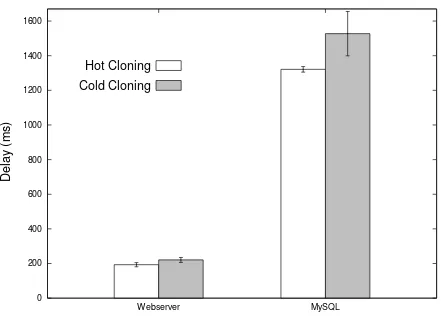
Figure 4.6 shows the comparison between the average delay after hot cloning and cold
cloning for different applications. We chose a stateful application (MySQL database server)
and a stateless application (Webserver) to understand the advantage of both hot cloning and
cold cloning. We use only the average delay observed after cloning to eliminate the influence
of the cloning period. The experimental setup is similar to the RUBiS setup as mentioned in
section 4.1. The duration of the training period was 1800 seconds. The average delay observed
after hot cloning is better than cold cloning in both cases due to the warm cache. However,
the advantage of hot cloning is very less in a webserver due to its stateless nature. In MySQL,
we can see the real impact of hot cloning. MySQL database used in our experiment caches the
index of the entire table. We take advantage of the hot cloning to reduce the overall warmup
time of the MySQL application. In the following paragraphs, we will compare the hot cloning
0 200 400 600 800 1000 1200 1400 1600
Webserver MySQL
Delay (ms)
Hot Cloning
Cold Cloning
0 200 400 600 800 1000 1200 1400
0 500 1000 1500 2000 2500 3000
Delay (ms)
Time (s)
25000
Cloning
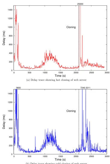
(a) Delay trace showing hot cloning of web server
0 200 400 600 800 1000 1200 1400
0 500 1000 1500 2000 2500 3000
Delay (ms)
Time (s)
7240
3800 2011
Cloning
(b) Delay trace showing cold cloning of web server
The input curve has a recurring pattern and as we can see in Figure 4.7a there is an
increase in average delay starting at 900 and lasts till 1500. When it tries to repeat itself at
2100, CloneScale predicts the increase in resource usage and triggers cloning (hot cloning in
this case). After a brief cloning period, we find that the SLO average delay is brought back to
normal. This clearly states the advantage of using CloneScale, which distributes the workload
among multiple nodes when the resource demands of a VM exceeds the resource available on
that physical host. Figure 4.7b shows the average delay trace of a web server performing cold
cloning. In order to compare the effect of hot and cold cloning, we used the same input trace
for both the experiments. Similarly near 2100, CloneScale predicts the increase in resource
demands and triggers cold cloning. In cold cloning the running VM is never stopped and a new
VM is started from a template, but still we observe a single huge peak. This is due to the load
balancer. After adding a new node to the haproxy load balancer we have to restart the load
balancer for the change to take effect. Even though, the restart takes only one or two seconds,
the system drops all the incoming packets during that period. We can overcome this issue, by
replacing the haproxy load balancer with another load balancer that supports dynamic addition
of nodes. CloneScale is independent of the load balancer and can work with any load balancer.
Finally, Figure 4.7 shows the average delay between 2140 and 2800 seconds. This average delay
observed after hot and cold cloning are roughly the same. Cold cloning observes a small warmup
time right after cloning, but when we consider the average delay between 2000 and 2800 seconds
(including the time taken for cloning), cold cloning does better than hot cloning due to its small
cloning phase. Since time taken for cold cloning is less and the difference in delay after cloning
is only slightly greater than hot cloning, it is more apt for cloning web server.
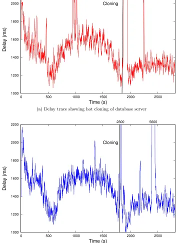
Figure 4.8 shows the comparison between hot and cold cloning of a database server. The
RUBiS setup includes three web servers and one database server. The three web servers are
provided with three cores each and adequate memory to avoid bottleneck in this tier. In order
to create a bottleneck in the database tier, we used a very high workload with 1000 worker
1000 1200 1400 1600 1800 2000 2200
0 500 1000 1500 2000 2500
Delay (ms)
Time (s) Cloning
16100 2300
(a) Delay trace showing hot cloning of database server
1000 1200 1400 1600 1800 2000 2200
0 500 1000 1500 2000 2500
Delay (ms)
Time (s) Cloning
2300 5600
(b) Delay trace showing cold cloning of database server
0 500 1000 1500 2000
1200 1400 1600 1800 2000 2200 2400
Delay (ms)
Time (s)
cold cloning hot cloning
sure the model can view the recurring pattern and make accurate predictions. In Figure 4.8a,
hot cloning is triggered at the 1850th second and lasts for a duration of 44 seconds. The figure
also shows the reduction in average response time after cloning. Figure 4.8b shows the impact
of cold cloning on the database tier. In cold cloning, we create a cloned VM from a template
and thus we will miss all the stateful application specific information available in the memory.
We used the pmap linux command to check the memory footprint of the MySQL process. We
found that the VM cloned using hot cloning has a memory foot print of 396MB and the memory
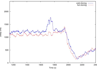
foot print of the VM cloned using cold cloning has a memory foot print of 164MB. Figure 4.9
shows the warmup phase observed in cold cloning. The delay trace of cold cloning is clearly
greater than the delay trace of hot cloning from 1150 seconds to 2100 seconds. After 2100
seconds, we find both curves are similar and this indicates the end of the warmup phase. The
warmup phase varies based on the application and its caching ability. We used MySQL myisam
database which stores the database index in the memory. From Figure 4.6 and Figure 4.9, we
understand the advantage of using hot cloning over cold cloning for stateful applications.
Figure 4.10 shows the progress of a Hadoop map node. This experiment was started with
two nodes, one master node and one slave node. The HDFS replication factor is set to 1 in
this experiment. The master node performs only reduce tasks and the slave node performs only
map tasks. Usually the same node performs both map and reduce tasks, we separated the VMs
performing map and reduce tasks to facilitate VM cloning. Wordcount on 282 text files was
used as the benchmark job to trace the progress rate. In Figure 4.10 , x axis denotes the time
in seconds and y axis denotes the progress in percentage. The progress rate is sampled every
five seconds using the Hadoop API. The progress rate of map node is nearly constant, around
0.72% every second. Whereas, the reduce node progresses 66% in the last few seconds and has
only 33% progress from the beginning, hence it is not an ideal candidate for cloning. Unlike
a web server or a database server, the CPU usage of a hadoop map node is mostly above 90
because it keeps performing map tasks as long as they are available. Thus, CloneScale cannot
0 20 40 60 80 100
0 20 40 60 80 100 120 140
Progress (%)
Time (s) Cloning
Without cloning Hot cloning
0 20 40 60 80 100
0 20 40 60 80 100 120
Progress (%)
Time (s) Cloning
Hot cloning Cold cloning
can use the Hadoop progress rate and estimated completion time to trigger cloning. In this
experiment, we trigger cloning manually to show that CloneScale can work with Hadoop. In
Figure 4.10, we manually trigger hot cloning at 120 seconds , During the cloning period (50s)
the Hadoop progress rate is zero. Once the cloning is completed, the map phase accelerates
as expected with the help of two mapper nodes. Figure 4.11 shows the comparison between
hot and cold cloning. The cold cloning is triggered at 120 seconds, since the running VM is
not stopped to save the state, the newly cloned VM joins the running VM which proves more
efficient as expected.
From our previous experiments we have identified that the power consumed by an idle
server is huge compared to the power used by the server under maximum CPU usage [24]. It is
better to consolidate and turn off or put the unused machines to sleep for saving power. Thus
it is very important to reduce the size of the application cluster when the cluster is not fully
utilized. CloneScale performs down-scaling to reduce the size of the tier dynamically when
the CPU usage is below a minimal threshold. This minimal threshold is configurable, usually
the minimal threshold is chosen less than half the maximum threshold to make sure there is
no fluctuation or no cloning right after down-scaling. This experiment shows the impact of
down-scaling by CloneScale compared to resource overprovisioning.
The same RUBiS setup was reproduced on the HGCC cluster. To illustrate down-scaling
we created an initial system with two RUBiS web servers and two RUBiS database servers.
The client generator generates workload that can be easily satisfied with just one node. After
the training phase, CloneScale slave triggers down-scaling and the web servers count is reduced
to one. The minimum threshold for this experiment was set at 30. When the CPU usage was
predicted to go below 30, down-scaling is triggered. The prediction model was trained with 100
samples with two second sampling interval. During down-scaling, the VM is first removed from
the load balancer list and the load balancer is restarted. After a minute, if the VM is not used,
it is destroyed.
0 20 40 60 80 100 120 140 160
0 100 200 300 400 500 600 700 800
Total CPU (%)
Time (s)
Down-Scaling Cloning With CloneScale
Without CloneScale
(a) Total web server tier CPU usage
0 50 100 150 200
0 100 200 300 400 500 600 700 800
Delay (ms) Time (s) 2800 520280 Down-Scaling Cloning With CloneScale Without CloneScale
(b) Delay trace - cold cloning
0 10 20 30 40 50 60 70 80 90 100
Over-Provisioning CloneScale
Average Delay (ms)
and its usage goes below the minimal threshold, a down-scaling request is sent to the master
node but the master node ignores this request because there is only one node left in that tier. At
510 seconds, when the predicted CPU usage exceeds the upper threshold (80% in this case), we
trigger cloning again. Since, we are working with the web server tier, we perform cold cloning.
In figure 4.12a, we have demonstrated both down-scaling and cloning and also compared it with
the over provisioned trace to show the change in trend. Figure 4.12b shows the delay tarace of
a VM. We can see that we have reduced the resource usage with a small increase in delay. The
spikes after the cloning phase are due to the warmup phase of cold cloning. To confirm it is the
warmup phase, we repeated the same expeirment with hot cloning. Figure 4.12c shows that
there is a brief cloning period with very high delay. After the cloning phase, we see an increase
in average delay of the CloneScale case compared to without CloneScale case. This is due to
the incremental QCOW2 images created during hot cloning. The without CloneScale trace is
collected from VMs that are created from base QCOW2 images. We did further experiments
to confirm the increase in average delay after cloning is due to the incremental QCOW2 image
and not the cloning itself. Figure 4.13 proves that the performance of CloneScale using the cold
cloning is comparable and only slightly greater than over-provisioning.
Prediction is not very accurate. If there is a prediction mistake, a new node has to be
cloned to satisfy the deficit caused by the recent down-scaling, which is costly. To overcome
this situation, on a down-scaling request, we remove the server’s IP from the load balancer but
leave the VM dangling for a minute before shutting down the VM. Having a VM as standby
Chapter 5
Related Work
In this chapter, we provide a brief survey of existing cloud scaling systems with more emphasis
on work related to VM cloning, migration and deployment.
In our previous work, CloudScale [24], we present an elastic resource scaling system driven
by prediction. Cloudscale employs online VM resource demand prediction as well as prediction
error handling in order to provide accurate resource to the VM. CloudScale does not address
adding or removing nodes to an existing application. In this thesis, we present CloneScale an
extension of CloudScale that distributes the workload among multiple nodes with the help of
VM cloning and load balancing to minimize the application SLO time.
In security, the Potemkin project [27] uses a dynamic VM creation technique to improve
honeypot scalability. On the arrival of network packets, a gateway router dynamically binds IP
addresses to physical honey farm servers. For each active IP address, Potemkin dynamically
creates a VM from a reference image. It implements copy-on-write optimization called delta
virtualization where the cloning operation maps all memory pages from the reference image.
The memory of reference image will be read only and all further write requests will be performed
locally. This helps in creating quick short-lived VMs but with one constraint that the newly
created VMs should share the same host with the reference image.
VM forking technique. In Snowflock, the application running inside the VM uses the fork API
to trigger cloning. While cloning, a VM descriptor containing the page tables, global descriptor
tables, metadata, VCPU register values and few memory pages is transferred from the parent
host to the clone host. The cloned VM is started with this VM descriptor and all initial read
requests by the child VMs are faulted and fetched from the parent VM. The newly cloned
VM will be in a virtual private network with parent and other child VMs. This design is
extremely effective to create quick clones with state but it needs to modify the VMM, host OS
and application running on the guest to use the API.
Kaleidoscope [4] uses snowflock to create swift transient short-lived VM clones for handling
bursts in workloads. As per snowflock implementation, the newly cloned VM will have large
number of page faults at the beginning, leading to a huge warm-up time. This design is not
suitable for handling bursts in workloads. Thus, kaleidoscope uses VM introspection techniques
to perform VM state coloring through which they identify the working set of the memory pages
and push the working set along with the VM descriptor to create a clone. The clone VM
created avoids the warm-up time and start servicing requests immediately. The kaleidoscope
architecture consists of the parent VM, multiple child VMs and also a gateway VM that
inter-faces the cluster to the outside world and performs load balancing. It monitors the number of
incoming client requests and spawns new worker clones when a defined threshold is exceeded.
Kaleidoscope discusses mainly about the cloning mechanism and gives more importance to
cre-ate short-lived VMs to handle bursts. Whereas, CloneScale concentrcre-ates more on the policy,
which determines when cloning should be initiated and what are conditions influencing the
decision. Kaleidoscope has addressed many shortcomings of Snowflock and tailor made the
implementation to support micro elasticity but it still needs to make changes in the VMM and
host OS. Whereas using CloneScale, we can perform VM cloning without making any changes
to the VMM or host OS. We also use a more intelligent scaling policy involving VM demand
prediction to trigger cloning before the application suffers from resource unavailability.
5, 3]. Chieu et al. [7] provide a solution to increase the scalability of webservers by monitoring
the number of incoming requests to each webserver and create a new webserver from a modified
image template when the number of requests increases above a threshold. Similarly when the
number of requests falls below a minimal threshold, unnecessary VMs are removed. Flurry
DB [19] uses Snowflock to create VM clones to dynamically scale the database tier. The load
balancer is designed to redirect read requests to any one clone and write requests to all clones.
This distribution technique makes sure all database are in a consistent state. During cloning,
the requests are queued in the load balancer and the queued requests are satisfied after cloning
completion. Harold et al [18] from Duke university presented an automated controller for
elastic storage system that uses control theory to determine the number of systems required
in the storage tier. Dolly [5] uses prediction techniques to predict the future workload and
performs cloning using VM snapshotting to scale the database tier. Dolly assumes there is
no shared storage between the servers, thus VM snapshots are transferred to the destination
server through the network. It takes into consideration the time taken for snapshotting and
replica resynchronization time during resource provisioning. CloneScale can perform cloning to
any application with minimal application knowledge and support from the user. We provide a
general user interface to the user for specifying the nature of the application and a script to
make application specific changes after cloning.
Few other related works such as Jump start cloud[30] and Rethink the Virtual Machine
Template [29] mainly concentrate on the quick deployment of VMs in the cloud environment.
Jump start cloud[30] discusses about deploying a VM from a template. The cloning mechanism
provided in this paper is similar to our cold cloning. It focuses only on VM deployment instead
of application scaling and does not address the problem of scaling policy. Rethink the Virtual
Machine Template [29] discusses about rapid deployment of stateful VMs. It avoids long VM
creation time by saving the VM state into a VM substrate, and then restore a new VM from the
substrate pool. Before saving a VM, it shrinks the VM memory size, detaches the devices, so
format and solves the issue associated with incremental qcow images by copying information
from the base image in background. This paper doesnt address the challenge of application
configuration and application scaling.
Live VM migration [16, 13, 12] has been the most famous solution provided to overcome
scaling conflicts among co-allocated VMs. ”Live migration of VMs” [16] provides a technique
to migrate a VM from one host to another without any downtime. In live migration, resources
are reserved on a destination host and VM memory pages are copied from source to destination.
Subsequent iterations copy only the recently dirtied pages. After transferring all the memory
pages, the VM is suspended at the source, its CPU state and remaining inconsistent memory
pages are transferred to the destination. After transferring the entire VM state successfully,
the original VM is discarded at the source and the destination activates the VM. The duration
of live migration depends on two important factors, the memory size and the memory access
rate. For a memory intensive VM, it takes multiple iterations to transfer the entire memory
content to the destination. Other existing solutions [13, 12] aim at providing post-copy based
live migration. Here, the VM is first transferred to the destination by copying its CPU state
and important memory pages. Further memory pages are fetched after each page fault. The
post-copy implementation helps in moving the VM out of a congested host before transferring
the memory pages but the VMM has to be modified to support post-copy migration. Previous
work, that suggests VM migrations as a solution to scaling conflict, assumes there are free hosts
available to migrate the VM. However, there are special scenarios where there are no better
physical hosts available or the VM requirement exceeds the resources available on that physical
host. CloneScale considers this scenario and aims at avoiding this limitation by distributing
the workload between multiple nodes.
Previous work has studied IO resource scaling in virtualized environment. Virtual IO
Sched-uler [23] provides a fair IO schedSched-uler by creating separate queues for each application. They
apply weight to each queue and schedule them according to Virtual IO scheduler (VIOS). The