An Examination of Individual Sequential Behavior Modeling in the Context of Healthcare Simulation.

(1)

ABSTRACT

TOWNSLEY, RACHEL MARIE. An Examination of Individual Sequential Behavior Modeling in the Context of Healthcare Simulation. (Under the direction of Maria E. Mayorga).

The application of quantitative and analytical methods in healthcare research has gained

consid-erable attention in recent decades as population health problems become more pronounced: aging

populations, growing costs, and growing health disparities. At the same time, political forces create

dynamic uncertainties in the structure and delivery of healthcare, while changes in technology and

medical science continually provide new insights that impact efficacy and outcomes. Increased

access and availability of data related to each of these components indicate tremendous

oppor-tunities for quantitative methods to make tangible impacts in improving the efficacy, efficiency,

and delivery of healthcare. However, quantitative models must be able to meaningfully capture

complex and interacting dynamics in order to offer practical insights to policy makers and other

stakeholders. Simulation modeling is a natural fit for this task as it provides a framework which can

capture dynamics of disease progression, population changes, and policy structures.

Simulation models of healthcare systems and processes are intrinsically linked to the "human

variable" which introduces a unique type of complexity. One specific aspect of this which is not

typically addressed in depth, is the modeling of individual behavior in healthcare contexts. Even

perfect models of disease progression, medical intervention efficacy, and population dynamics

are limited when simplifying assumptions are made about patient behaviors. In the context of

preventative care such as cancer screening, these patient behavior patterns heavily impact outcomes

and policy efficacy. The task of modeling patient behaviors is uniquely constrained by patient privacy

requirements as well as limited observation windows, particularly in transient and vulnerable

populations. Additionally, components of health beliefs, behavioral economics, and the notion of

individual agency each contribute to the complex nature of the challenge.

This dissertation work is focused on examining model approaches that address capturing

(2)

cancer. Three distinct modeling strategies are examined to generate synthetic screening behavior

trajectories for a simulated population: statistical classification, Markov chains, and survival

anal-ysis. These strategies are implemented using private insurance claims data for colorectal cancer

screenings as well as national survey data.

This research provides several frameworks for utilizing incomplete longitudinal data and

re-peated cross-sectional survey data to inform simulated individual behaviors, and characterizes

the challenges and implications of each approach. The findings show that the behavior models

implemented in population level healthcare simulations can have significant impacts on predicted

outcomes, and underscores the care that should be taken in choosing how to capture human agency

in these contexts. Policy recommendations derived from these types of simulations should be tested

(3)

(4)

An Examination of Individual Sequential Behavior Modeling in the Context of Healthcare Simulation

by

Rachel Marie Townsley

A dissertation submitted to the Graduate Faculty of North Carolina State University

in partial fulfillment of the requirements for the Degree of

Doctor of Philosophy

Industrial Engineering

Raleigh, North Carolina

2018

APPROVED BY:

Kristen Hasmiller Lich Min Chi

James Wilson Maria E. Mayorga

(5)

BIOGRAPHY

Rachel Townsley is a doctoral candidate in the Edward P. Fitts Department of Industrial and Systems

Engineering at North Carolina State University. Born in Hong Kong and raised trotting the globe,

Rachel received her Bachelor’s degree in Industrial Engineering from the University of Arkansas

prior to moving to Raleigh, but isn’t very southern. Her research interests are in quantitative models

of stochastic systems in application areas tied to human and societal welfare. After the completion

of her doctorate, Rachel will work as a Research Analyst in the Healthcare Research Policy team at

(6)

ACKNOWLEDGEMENTS

I am immensely grateful to my advisor, Dr. Maria Mayorga, for her unwavering support, supernatural

patience, and pragmatic guidance throughout the past five years. I so appreciate your willingness to

let me explore work that felt personally interesting and gratifying to me. Thank you for challenging

me, encouraging me, believing in me, and humoring me at each turn.

Thank you to my committee, Dr. Kristen Hassmiller Lich, Dr. Min Chi, and Dr. James Wilson

for their time, enthusiasm, guidance, and feedback, which has immeasurably improved this work

and has taught me so much. I have also appreciated and valued Dr. Stephanie Wheeler’s continued

interest and measured input in each of the research projects I have undertaken. Thank you to Dr.

Mike Carter for offering his expertise and feedback throughout the writing process.

I would not be the same without the friendships that were forged within the windowless walls of

Daniels 373/375. Nisha, Shakiba, Karen, Sidd, Lena, Katy, Joe, and Kendall . . . thank you all for the

companionship, commiseration, ridiculousness, weekend trips, cooking adventures, questionable

dance moves, and very serious collaborative research discussions. Thanks especially to Nisha and

Sidd, who are kindred spirits and have been sources of heartfelt support in turbulent times.

I hold several of my undergraduate professors responsible for my undertaking this doctorate: Dr.

Scott Mason, who made me much more interested in applied research than coursework, Dr. Ashlea

Bennett Milburn, who introduced me to healthcare systems research, Dr. Manuel Rossetti, from

whom I learned that simulation modeling is the solution to all of life’s problems, and Dr. John White,

the best academic grandfather anyone could ask for. I would not have ended up in graduate school

without their support and influence many years ago, and I am thankful.

Thank you to Jenn, whose love brightens each day, and whose care and encouragement have

greatly enabled the production of this dissertation.

Finally, thank you to my family. I will always be grateful to my parents, Lindel and SoonMee,

for their steadfast love and for raising me to be persistent, confront difficulty, and value sincerity.

Thank you to my brothers and sisters: Jared, Jason, Christine, and Rebekah, who are each curious,

diligent, reflective, and strong in ways that inspire me to be better. You are my longest friends and

(7)

BIBLIOGRAPHY . . . 99

APPENDIX . . . .108

(9)

LIST OF TABLES

Table 2.1 Payer Type Demographics . . . 13

Table 2.2 Demographic Statistics of Initial Population . . . 13

Table 2.3 Demographic Comparison of Commercial Population Before and After Exclu-sions . . . 21

Table 2.4 Statistics of screening prevalence is shown by subpopulation . . . 21

Table 2.5 Screening statistics by subpopulation. FIT/FOBT and Colonoscopy statis-tics denote the portion of the population who received a FIT/FOBT or a Colonoscopy within the 5 year observation time . . . 22

Table 3.1 Logistic regression estimates to predict the probability of compliance (receiv-ing a screen of any kind) for individuals observed for ages 50-54 . . . 27

Table 3.2 Logistic regression estimates to calculate the probability that an individual receives a colonoscopy as their first screen, for individuals observed between ages 50-54 . . . 28

Table 3.3 Estimated parameters for the multinomial logit model . . . 34

Table 3.4 Mean multinomial probit parameter estimates (default choice is No Screen) . . 36

Table 3.5 Mean predicted probability estimates from probit model vs logit probabilities 36 Table 3.6 Confusion Matrix for 5 fold cross validation for sequential binary logistic re-gression . . . 39

Table 3.7 Confusion Matrix for 5 fold cross validation for multinomial logistic regression 40 Table 4.1 Markov order test statistics and results for the age 57 strata . . . 47

Table 4.2 Sample third order transition probabilities for age 57. Highlighted rows are transition probabilities which are estimated based on 10 or less transitions observed in the data set. For these transitions we force the transition to to "N" state with probability 1. . . 49

Table 4.3 Sample 2nd order transition probabilities stratified by gender and geography . 50 Table 4.4 Confusion Matrix for predicting the 5th screening behavior for 3rd Order Ho-mogeneous Markov chain model . . . 52

Table 4.5 Confusion Matrix for predicting the 5th screening behavior for 2nd Order Stratified Markov chain model . . . 52

Table 5.1 CRC Screening Questions in the BRFSS Questionnaire . . . 56

Table 5.2 List of variables initially included in the preferred modality logistic regression 57 Table 5.3 Logistic regression estimates to predict P(preferred modality=colonoscopy) based on BRFSS survey responses . . . 57

Table 5.4 Variables used to evaluate demographic similarity between states . . . 61

Table 5.5 Top ten states ranked by similarity to Oregon . . . 62

Table 5.6 Estimated diffusion curve parameters . . . 64

Table 5.7 Possible Responses in the BRFSS Questionnaire (Time since FIT/FOBT) . . . . 66

(10)

Table 5.9 Estimated screening rates based on BRFSS survey and insurance claims data, under the assumption that the time between screenings is exponentially

dis-tributed . . . 69

Table 6.1 Summary of necessary assumptions about the nature of screening behavior for each modeling approach . . . 77

Table 6.2 Types of heterogeneity captured in each modeling approach . . . 78

Table 6.3 Distribution of partial trajectory types in the empirical data . . . 83

Table 6.4 Chi Sq Test statistics comparing each behavior model outcomes to the empiri-cal data . . . 83

Table 6.5 Cluster membership of unique cumulative years UTD trajectories . . . 94

Table A.1 Second Order transition probabilities for ages 52-55, stratified by gender and geography (FR: female, rural; MR: male, rural; FU: female, urban; MU: male, urban) . . . 110

Table A.5 Third Order transition probabilities for ages 53-58 . . . 114

Table A.6 Third Order transition probabilities for ages 59-64 . . . 115

(11)

LIST OF FIGURES

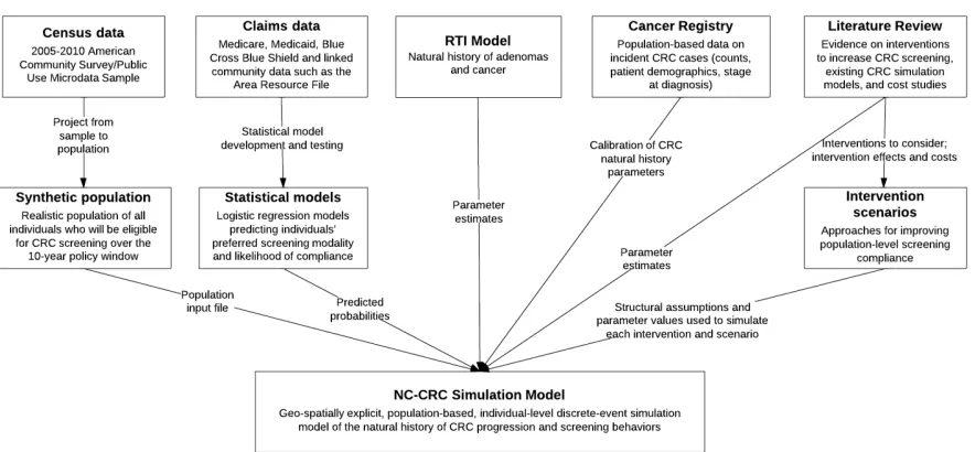
Figure 1.1 NC-CRC simulation model inputs . . . 7

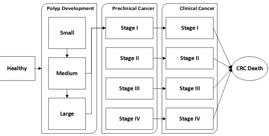
Figure 1.2 NC-CRC simulation natural history progression . . . 8

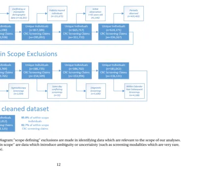
Figure 2.1 Data Exclusions Diagram:"scope defining" exclusions are made in identifying data which are relevant to the scope of our analyses. Additional exclusions "within scope" are data which introduce ambiguity or uncertainty (such as screening modalities which are very rare, conflicting screening records). . . 12

Figure 2.2 Count of observed by quarter . . . 14

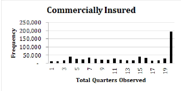
Figure 2.3 Distribution of quarters observed for each individual (Commercially Insured) 14 Figure 2.4 Distribution of quarters observed for each individual (Publicly Insured) . . . . 15

Figure 2.5 Data densities by age for commercially insured . . . 16

Figure 2.6 Data densities by age for publicly insured . . . 16

Figure 2.7 Histogram of time between FIT/FOBT and subsequent colonoscopy . . . 19

Figure 2.8 The percent of the observed population receiving a CRC screening by Age for commercially insured individuals in the final data set . . . 22

Figure 3.1 Effects plot for compliance logistic regression . . . 27

Figure 3.2 ROC for compliance prediction model . . . 28

Figure 3.3 Effects plot for modality logistic regression . . . 29

Figure 3.4 ROC Curve for Modality Prediction Model . . . 29

Figure 3.5 Choice structure for the sequential logistic regression modeling approach . . . 31

Figure 3.6 Choice structure for the multinomial logistic regression modeling approach . 32 Figure 3.7 Effects plots for multinomial logistic regression . . . 35

Figure 3.8 ROC curve for multinomial logistic regression model . . . 35

Figure 4.1 number of observed transitions available to estimate the parameters needed for each order Markov chain . . . 45

Figure 4.2 Transition diagram for the 2nd order model. Each transition is informed by a age specific transition matrix. . . 51

Figure 5.1 Effects plots for predictors of colonoscopy as a preferred modality . . . 58

Figure 5.2 ROC Curve for the preferred modality prediction model . . . 59

Figure 5.3 National empirical ever-screened rates by birth cohort and age . . . 60

Figure 5.4 Ever Screened rate comparisons for the 1945-1949 birth cohort. We compare the rates for the state of Oregon, Oregon combined with Washington, Oregon, Washington and other similar states (as identified in the similarity analysis) and National. . . 63

Figure 5.5 Fitted diffusion curves are compared to the empirical data for each birth cohort, where the orange line is the fitted diffusion curve, empirical points are in blue, and the probability distribution of age at first screen is shown in gray (right axis). . . 65

(12)

Figure 5.7 Estimated survival curve for time until next colonoscopy based on the fitted

λusing BRFSS survey responses . . . 70

Figure 5.8 Estimated survival curve for time until next FIT/FOBT based on the fittedλ

using BRFSS survey responses . . . 70

Figure 5.9 Estimated survival curve for time until next FIT/FOBT based on the fittedλ

using Oregon claims data set . . . 71 Figure 5.10 Screening behavior as implemented in a simulation model using the Survival

Analysis strategy . . . 72

Figure 6.1 The percent of the population receiving a colonoscopy screening (by age).

The figure shows colonoscopy incidence across ages for each modeling imple-mentation, as well as the empirical incidence seen in the partially censored claims data . . . 80

Figure 6.2 The percent of the population receiving a FIT/FOBT screening (by age). The

figure shows FIT/FOBT incidence across ages for each modeling

implementa-tion, as well as the empirical incidence seen in the partially censored claims data . . . 81 Figure 6.3 The percent of the population by age, that has received a FIT/FOBT test within

the last year, or a colonoscopy within the last 10 years. The entire lifecourse of the population was simulated from birth to death, with death age capped at 100 85 Figure 6.4 The percent of the population by age, that has received a FIT/FOBT test within

the last year, or a colonoscopy within the last 10 years . . . 87

Figure 6.5 Histograms of the number of screenings received per individual for each

screening behavior model . . . 89 Figure 6.6 Implicit CRC screening diffusion for each modeling approach . . . 90

Figure 6.7 Screening Trajectories and Cumulative Years UTD trajectories for 4 example

individuals. Individual 1 receives FIT/FOBT screenings on even age years

(ages 50,52,54,...,64). Individual 2 receives FIT/FOBT screenings on odd age years (ages 51, 53, 55,...,65). Individual 3 receives a FIT/FOBT screening every year. Individual 4 receives no screenings at all. . . 92

Figure 6.8 Standardized criterion related to cluster quality, for each number of clusters

under consideration. Based on these criteria, we select k=6 . . . 93 Figure 6.9 Graphs of each cluster of cumulative UTD trajectories . . . 95 Figure 6.10 The distribution across these trajectory type clusters for each screening

(13)

CHAPTER

1

INTRODUCTION

1.1

Motivation

Simulation models are powerful tools in stochastic process analyses as they provide a flexible

framework in which to capture and integrate the dynamics of complex, interrelated systems. These

dynamics can be difficult to incorporate into more traditional and analytic optimization modeling

methodologies like Markov decision processes and linear programming as these methods are often

mathematically or computationally limited[Chung, 2003; Robinson, 2004]. As computing power

becomes increasingly accessible, simulation based analyses have grown in popularity as a tool for

descriptive and predictive analysis of both manufacturing and service systems. The simulation

framework can easily incorporate other types of models and analyses as inputs, allowing for smooth

integration of multiple methodologies and interacting process components. This synthesis is often

(14)

act as a test-bed for recommendations garnered from a variety of quantitative analyses.

The application of quantitative and analytic methods in healthcare research has gained

consid-erable attention in recent decades[Brailsford et al., 2009]as population health problems become

more pronounced: aging populations[CDC, 2003], growing costs[Bodenheimer et al., 2009], and

health disparities[Lasser et al., 2006]. At the same time, political forces create dynamic

uncertain-ties in the structure and delivery of healthcare, while changes in technology and medical science

continually provide new insights that impact efficacy and outcomes. Increased access and

availabil-ity of data related to all of these components indicate tremendous opportunities for quantitative

methods to make tangible impacts in improving the efficacy, efficiency, and delivery of healthcare.

However, these quantitative approaches must be able to capture complex and interacting

dynam-ics. Simulation modeling is a natural fit and is an increasingly popular approach for these types

of quantitative analyses[Brailsford et al., 2009; Fone et al., 2003; Mustafee et al., 2010; Pitt et al.,

2016; Tunnicliffe-Wilson, 1980], providing a framework which can capture dynamics of disease

progression, population changes, and policy structures.

These types of simulation models are intrinsically linked to the “human variable” which

in-troduces a unique type of complexity. One specific aspect of this which is not often addressed

in depth, is the modeling of individual choice and behavior in healthcare contexts. Even perfect

models of disease progression, medical intervention efficacy, and population dynamics are limited

in the insights they can provide when simplifying assumptions are made about patient choices and

behaviors. The task of modeling patient behaviors is uniquely constrained by data access due to

patient privacy requirements as well as limited observation windows, particularly in transient and

vulnerable populations. Additionally, components of health beliefs, behavioral economics, and the

notion of individual agency each contribute to the complex nature of the challenge.

Within the healthcare realm, one critical health behavior which has a direct and significant

impact on health outcomes is cancer screening. In the United States, three types of cancer screening

are supported by the Centers for Disease Control and Prevention (CDC) as having evidence for

(15)

cancer, and colorectal cancer[Mählck et al., 1994; Nelson et al., 2009; Welch & Robertson, 2016]. These

screenings are recommended to occur over significant portions of individual lifespans (ages 21-65

for cervical cancer, 50-75 for breast and colorectal cancers), and require repeated screening events

at regular intervals. A recent study demonstrates the sensitivity of policy outcomes to breast cancer

screening compliance, concluding that it is important for screening recommendation adherence

behaviors to be explicitly considered in the evaluation of policy recommendations and interventions

[Ayer et al., 2015].

In this dissertation we focus on models of colorectal cancer screening behavior, though we

believe that much of the work is generalizeable and can translate readily to other screening contexts.

1.2

Health Behavior in Simulation Models

In healthcare contexts patient behavior plays a critical role in determining health outcomes. The

efficacy of treatments and policy interventions is not only dependent on individual biology and

physiology, but also on the patient preference of modality as well as the patient’s compliance

behav-ior. This has implications in many areas of healthcare including screening for common diseases

(CRC, breast cancer, cervical cancer, diabetic retinopathy, etc.) as well as medication use (oral

contraceptives, smoking cessation aids, mood stabilizers and antidepressants). It is therefore

impor-tant to consider the ways these behaviors are modeled in simulation studies which examine these

phenomenon.

In health psychology there are several theoretical models of health behavior, including Becker’s

Health Belief Model[Becker, 1974], Ajzen’s Theory of Planned Behavior[Ajzen, 1991], Walston’s

Health Locus of Control Model[Wallston et al., 1978], and Schmidt’s Physical, Emotional, Cognitive,

and Social (PECS) Model[Schmidt, 2000]. These models are focused on explaining health related

behaviors of individuals based on a combination of their internal attitudes, beliefs, and psychological

processes. Sally Brailsford et al.[Brailsford & Schmidt, 2003; Brailsford et al., 2012]explore the

incorporation of some of these models in a healthcare simulation context, but notes that these

(16)

the implementation of psychological models of health behavior in simulation is compelling, it is

inevitably limited in scope as there is no way to meaningfully access the data necessary to inform a

representative, population level simulation analysis.

In the design of simulation models focused on developing screening policies and

recommen-dations, the task of capturing stochasticity is often focused on aspects of disease progression,

population dynamics, and screening efficacy, while assuming 100% compliance[Knudsen et al.,

2016; Zauber et al., 2009]. These models offer critical insights into optimizing best case outcomes,

but can be limited in accurately capturing or predicting outcomes when impacted by practicalities

of policy implementation. Other studies do cost-effectiveness analyses at various fixed

compli-ance levels[Frazier et al., 2000; Mandelblatt et al., 2009; Stout et al., 2006]. These models fail to

address heterogeneity in health behaviors, making it difficult to capture subpopulation outcomes

and disparities.

Many public health studies investigate cancer screening compliance trends and offer important

insights identifying predictors of screening behavior. These studies utilize a variety of data sources

including survey data, hospital data, and insurance claims data. These data sources are subject

to varying limitations. Although these studies provide insights into compliance rates, modality

selection, and predictors of behavior, they do not clearly translate into obvious implementation

strategies in a modeling context. These studies do demonstrate important aspects of screening

behavior to be considered, namely that compliance and modality selection varies accross

popula-tions (socio-economic satus, insurance status, race, sex, geography, age) and that prior screening

compliance is often correlated with future compliance[Denberg et al., 2005; Gwak, 2016; Hawley

et al., 2008; Riekert et al., 2013; Sohl & Moyer, 2007; Subramanian et al., 2004]. There are a handful of

simulation model analyses which incorporate predictive models from the medical literature (such

as[Gierisch et al., 2010]in[Tejada et al., 2014]). These are discussed in more detail in Chapter 3.

In this dissertation we focus on modeling modality choice and recommendation compliance in

(17)

1.3

Colorectal Cancer

Colorectal cancer (CRC) is one of the leading causes of preventable death in the United States.

Although it is often treatable with early detection, around 51,000 individuals die from CRC annually

[United States Cancer Statistics: 1999-2014 Incidence and Mortality Web-based Report]in the United

States. It is the second most prevalent type of cancer affecting both men and women, and accounts

for 8.4% of all cancer related mortality[Cancer Stat Facts: Colon and Rectum Cancer]. Additionally,

the financial burden of the disease is substantial, accounting for close to 12% of all cancer treatment

expenditures in the United States. Estimates range from $4.5 to $9.6 billion for annual CRC treatment

costs[Yabroff et al., 2009].

Treatments for CRC are effective when detected early, and screening can also prevent cancer

cases through the removal of precancerous polyps[Bibbins-Domingo et al., 2016]. An estimated

57% of stage I CRC cases survive 10 years after diagnosis. In contrast, only 7% of stage IV cases

survive past 10 years post diagnosis[Soerjomataram et al., 2012]. This underscores the importance

of screening and early detection and its potential to reduce CRC incidence and mortality.

For average risk asymptomatic patients the US Preventive Services Task Force recommends

screening from age 50 to 75, with multiple modalities available which have varying recommended

frequencies. If an individual has been screened within a time period less than the recommended time

between screens for a given modality, the individual is considered "up to date" with respect to CRC

screening. Screenings occur in two different modality types: stool based tests and direct visualization

tests. Among stool based tests are the fecal occult blood test (FOBT) and the fecal immunochemical

test (FIT). Both of these tests are simple, inexpensive stool sample tests which can be collected in the

comfort of a patient’s home with a kit and then mailed to a lab. An annual frequency is recommended

for these modalities, so an individual is considered up to date only if they have received one of these

screenings within the past year. Direct visualization tests such as colonoscopies, colonographies,

and flexible sigmoidoscopies generally require less frequent screening to be up to date. While they

(18)

comprehensive screening modality. Among this screening type, colonoscopies are most frequently

utilized, with a recommended frequency of 10 years[Bibbins-Domingo et al., 2016].

Despite these screening recommendations, approximately 35% of age eligible individuals in the

United States were not up to date in 2012, and 27.7% reported that they had never been screened.

[Vital Signs: Colorectal Cancer Screening Test Use]. The CDC estimates that 60% of all CRC mortalities

can be averted by following recommended screening policies[CDC, 2013]. The prevalence of non

compliance and inconsistent compliance in the context of population level CRC simulation models

becomes relevant in modeling patient behavior as it is significantly impacted by patient and provider

characteristics[Hawley et al., 2014; Inadomi et al., 2012; Wheeler et al., 2017]and plays such a

significant role in health outcomes.

We utilize a population level microsimulation model, NC-CRC[Lich et al., 2017]which

simu-lates the entire life course of each individual in a state population and tracks polyp and adenoma

progression and associated CRC outcomes such as up-to-date with screening, diagnosis, incidence,

and treatment while incorporating screening, insurance, and treatment dynamics. Simulation

com-ponents and their associated input data sources are illustrated in Figure 1.1. In the model logistic

regressions are used to predict modality and compliance components of patient behavior based on

claims data.

The natural history component of the model is adapted from a model built by RTI[Subramanian

et al., 2009]and informed by disease progression and incidence rates from[Loeve et al., 2000],

summarized in Figure 1.2.

1.4

Current Practices in CRC Screening Models

Although there are several simulation models and Markov models aimed at predicting and evaluating

the impact of CRC policies, few publications detail the screening behavior modeling aspect.

Three CRC simulation models are currently included in the Cancer Intervention and Surveillance

Modeling Network (CISNET) which is a consortium of quantitative models developed by

(19)

Figure 1.1NC-CRC simulation model inputs

in its original implementation estimated individual compliance probabilities to be dependent on

compliance history, where prior compliance implies a higher compliance rate in the next screening

round. The total percentage of the population modeled as compliant was held constant over time.

In the SimCRC model[SimCRC Profile], base compliance rates were estimated from NIH survey

data based on age, sex, race, and calendar year, and then categorized into low, moderate, or high

compliance. Finally, the CRC-SPIN model[Rutter & Savarino, 2010]ignores stochasticity in screening

behavior, measuring outcomes under the assumption of perfect compliance.

Additionally, other noteable CRC Models appear in the literature[Council, 2005]. In the Harvard

model[Frazier et al., 2000]initial screening in the FOBT modality is assumed to be 60% and follow up

screening (colonoscopies) are assumed to be 80% compliant, independent of previous compliance.

The Ladabaum Model[Ladabaum et al., 2004; Song et al., 2004]and similarly the Vijan Model[Vijan

et al., 2001]assigns a set percentage of the simulated population to either be fully compliant to

recommended screening throughout their lifetime, or fully noncompliant. Lastly, in the Vanderbilt

Model screening adherance is assumed to be 70% overall, with patient characteristic adjustments

(20)

Figure 1.2NC-CRC simulation natural history progression

1.5

Research Objectives

The goal of this dissertation is to characterize strategies for modeling patient behavior in healthcare

simulation models, specifically repeated behaviors such as cancer screening. We examine this in the

context of colorectal cancer screening where multiple screening modalities are available, utilizing

limited data from insurance claims and national survey data. We consider the limitations and

assumptions inherent in each of the approaches and demonstrate that the implications of behavior

model choice can be significant in the context of population predicted outcomes.

The contents of this dissertation are as follows. Chapter 2 provides an overview of an insurance

claims data set which is used in Chapters 3 and 4. This chapter is intended to familiarize the reader

with the contents and format of the data as well as providing descriptive statistics regarding CRC

screening and offering insight into data exclusion decisions. In Chapter 3 patient screening behavior

is modeled using statistical classification in two choice structures. In the first, the behavior is modeled

using two binary classifiers in sequence, one which predicts the patient’s modality, and the second

(21)

as a "modality choice" and a multiclass classifier is used to predict individual screening behavior

as FIT/FOBT, colonoscopy, or None. In Chapter 4, two Markov chain models are used to predict

individual screening trajectories. One Markov chain model uses 3rd order transition probabilities

to predict behaviors as an individual ages (treating the population as behaviorally homogeneous),

while the second uses second order transition probabilities stratified by gender and geography in

order to introduce heterogeneous behavior into the population. In Chapter 5, we incorporate a

separate data set from preceding chapters, using national survey data to inform a survival modeling

approach to generate screening trajectories. Screening behavior is modeled in 3 components:

modality preference, time until first screen, and time between subsequent screenings. Finally, in

Chapter 6, we conduct comparative analyses and discuss the implications of each approach with

(22)

CHAPTER

2

CLAIMS DATA OVERVIEW

The primary dataset used in this dissertation is extracted from claims data owned by Oregon Health

and Science University. Claims data is based on records of reimbursement requests made to

in-surance providers when medical procedures are conducted, and contain procedure codes which

were used to identify CRC screenings. The dataset contains Oregon residents who are commercially

insured as well as publicly insured through Medicaid. Medicare claims data is not available. We

stratify the dataset by payer type as is common in many healthcare studies,under the assumption

that the populations are fundamentally distinct enough to warrant separate analyses.The data was

received in two parts. The first dataset contains descriptions of individuals and whether or not

they were under observation in a given calendar quarter. The second dataset contains screening

procedure date and modality. The two datasets are linked by an anonymized ID number.

A diagram of data exclusions and adjustments is shown in Fig. 2.1. An initial set of "scope

(23)

(eliminateing data based on age, insurance status, and observation period). Additionally we identify

and exclude screening data which introduce ambiguity or uncertainty (such as screening modalities

which are very rare, conflicting screening records). The following sections offer details of these

exclusions as well as descriptive statistics of the data set.

2.1

Observation Data

The data includes all individuals who are observed for ages relevant to colorectal cancer screening,

age 50 to age 75, who are observed during any calendar quarter between 2010 and 2014. For each

individual we have age, gender, and geographic status (urban or rural). For individuals publicly

insured through Medicaid, we have race data as well. In the Medicaid data, individuals are

classi-fied by race as Hispanic, non-Hispanic White, non-Hispanic African American, and non-Hispanic

Other/Unknown.

2.1.1 Initial Exclusions

The dataset captures observations of 835,590 individuals. Of these, 18,201 contain conflicting records

with regard to gender, race, or geography at different points in time, leaving 817,389 unique

indi-viduals with unconflicted data. While gender and race are invariant variables and are not expected

to change with time, geography may truly change. However, those with changes in geography are

removed for simplicity, as urban/rural classification is a sub-population of interest and is used as a

stratifying variable.

2.1.2 Demographic Statistics

Of the remaining individuals in the dataset 81.4% (n=665,717) are commercially insured and 18.6%

(n=151,672) are publicly insured through Medicaid (Table 2.1). For commercially insured individuals,

51.8% are female, and 65.6% live in urban geographical areas. Race data is not available for

commer-cially insured individuals. For publicly insured individuals, 53.0% are female and 56.6% reside in

(24)

(25)

Table 2.1Payer Type Demographics

Payer Type Count of Unique IDs

Commercial 665,717 81.44%

Medicaid 151,672 18.56%

Total 817,389

Table 2.2Demographic Statistics of Initial Population

Commercial Medicaid Commercial Medicaid

Gender Male 48.17% 47.01% 320,678 71,294

Female 51.83% 52.99% 345,039 80,378

Race White N/A 64.50% 97,827

African American N/A 2.81% 4,266

Hispanic N/A 11.64% 17,659

Other/Unknown N/A 21.05% 31,920

Geography Urban 65.55% 56.59% 436,404 85,833

Rural 34.45% 43.41% 229,313 65,838

are white, 2.8% are African American, 11.6% are Hispanic,and 21.0% are of an Other/Unknown race.

See Table 2.2.

2.1.3 Observation Statistics

Fig. 2.2 illustrates the number of individuals observed in the dataset over time. While the count

of commercially insured individuals remains relatively stable, we observe a sudden increase in

Medicaid individuals at the start of 2014. This is expected, as Oregon participated in the Medicaid

Expansion portion of the Affordable Care Act which was implemented in January of 2014. This raised

the minimum income thresholds required to qualify for Medicaid in the state of Oregon, resulting

(26)

Figure 2.2Count of observed by quarter

Fig. 2.3 and Fig. 2.4 show the distribution of the number of quarters observed for each individual.

For the commercially insured, about 29% (n=195,188) of individuals are observed for the full 5 year

observation window (20 quarters). In contrast, only 8% of publicly insured individuals are observed

for the full 5 years, while the majority (65%) are observed for 1 year or less. This is explained by the

dramatic increase in Medicaid enrollment due to Medicaid expansion in 2014

(27)

Figure 2.4Distribution of quarters observed for each individual (Publicly Insured)

Fig. 2.5 and Fig. 2.6 show the distribution of data densities by age at observation and calendar

quarter for commercially and publicly insured individuals respectively. In the commercially insured

population, a dramatic drop off in enrolled individuals is observed from age 65 onward as individuals

who have aged into Medicare eligibility are less likely to be commercially insured. This may also

imply an underlying difference in the population represented by data observed prior to age 65 versus

after 65, as individuals who opt to stay commercially insured after qualifying for Medicare are likely

meaningfully different than those who do not.

In the publicly insured Medicaid population there is no data for individuals age 65 or over,presumably

because Medicaid patients fully transfer to Medicare at age 65. Again, we observe that the majority of

Medicaid patients in the dataset for all ages are observed in the last four quarters of the observation

window in year 2014. This is due to Oregon’s Medicaid expansion under the Affordable Care Act,

(28)

Figure 2.5Data densities by age for commercially insured

Figure 2.6Data densities by age for publicly insured

Due to the limited observation continuity of the publicly insured population in our data set, we

opt to focus the analysis of this dissertation on the commercially insured. Further, because the shift

(29)

with individuals aged 65 and over. Descriptive analyses of the screening data for this population is

contained in the following section.

2.2

Screening Data

The screening data provided by the Oregon Health and Science University contains insurance claims

relevant to CRC screening. An adjusted date of service is provided, which is the actual date of service

toggled by a random number of days (uniform[-5,5]) in order to protect patient confidentiality. The

same service date adjustment is applied for all claims associated with a given patient in order to

preserve the sequence of screening claims. Claims are categorized in the dataset by procedure code

as either (1) colonoscopy, (2) FIT (specified), (3) FOBT (specified), (4) FIT/FOBT (nonspecified), or

(5) flexible sigmoidoscopy. We group the FIT/FOBT categories, reducing the screening claims to

either colonoscopy, FIT/FOBT, or sigmoidoscopy.

2.2.1 Initial Screening Data Exclusions

A total of 351,733 CRC screening claims records are tied to the 665,717 commercially insured

indi-viduals remaining after exclusions described in Section 2.1.1. Additionally, we exclude indiindi-viduals

who are aged 65 and over at the beginning of the observation period, leaving 624,171 individuals

tied to 336,267 CRC screening claims.

In order to utilize the most complete data points to characterize and model CRC screening

trajectories, we eliminate individuals who are observed for less than 5 continuous years. This

eliminates a significant number of individuals in the original data set, leaving 188,769 individuals

which are in our scope of interest (commercially insured, fully observed for the 20 quarters, under

the age of 65 at observation time). These individuals are associated with a total of 159,765 CRC

screening claims.

Of the within-scope data are claims for sigmoidoscopy procedures. Because this is relatively

rare in our dataset, and the prevalence of this procedure as a CRC screening modality is declining

(30)

sigmoidoscopy procedures from our dataset. Further, we eliminate 33 individuals who are tied to a

claim which is for two separate screening modalities in one day.

The final set of exclusions related to diagnostic versus routine screenings is explained in detail

in the following section.

2.2.2 Diagnostic Screening Exclusions

In the claims data used, we do not differentiate between routine screening colonoscopies

(colono-scopies which are performed with the intent of CRC screening only) from diagnostic screenings

(colonoscopies which are performed as a follow up after a patient experiences symptoms or has a

positive FIT/FOBT result). While different claims codes exist for different types of colonoscopies,

they are sometimes coded interchangeably as a colonoscopy initially intended as routine screening

can reveal polyps which can be removed during the same procedure, enabling the provider to bill

the procedure as diagnostic (which carries a higher reimbursement from insurance companies).

In this way, using claims codes to distinguish diagnostic from screening colonoscopies is

unre-liable, since we are interested in the intent of the screening behavior. However, there are cases in

the data where a colonoscopy claim is observed following a FIT/FOBT claim for a given patient. In

these cases, some colonoscopies are likely intended as diagnostic screenings, not routine

screen-ings, as FIT/FOBT results can indicate a problem and result in a recommendation for a diagnostic

colonoscopy. It is also possible that an individual may simply change CRC screening modalities.

According the screening recommendations, a negative FIT/FOBT result is only valid for 1 year before

repeated screening is recommended. Some individuals may screen FIT/FOBT one year, and decide

to undergo a colonoscopy the next year instead of continuing to screen FIT/FOBT annually.

In our data set we are interested in distinguishing cases where a colonoscopy follows a FIT/FOBT

screening for diagnostic reasons from cases where a colonoscopy follows a FIT/FOBT screening due

to a change in modality preference. Prior studies utilizing electronic medical records and laboratory

databases indicate that the majority of patients who follow-up a positive FIT/FOBT result with a

(31)

completion rate at 6 months and 83.2% within 12 months[Corley et al., 2017], while another study

finds completion rates of 50% within 6 months and 57.7% within 12 months[Martin et al., 2017].

We analyzed our claims data to evaluate whether a 6 month cutoff acts as a reasonable criteria

to differentiate diagnostic colonoscopies from routine screening colonoscopies that represent a

screening modality switch. Individuals with observed screening sequences that contain a FIT/FOBT

to colonoscopy transition, we calculate the time passed between these two screenings. Some

individ-ual screening sequences have multiple such modality switches; for these individindivid-uals we only analyze

the first such modality switch. In places where colonoscopies take place more than 12 months after

a FIT/FOBT, we assume these are screening colonoscopies as a FIT/FOBT screening is only valid

for 1 year before repeated screening is recommended. For the remainder, we look at the frequency

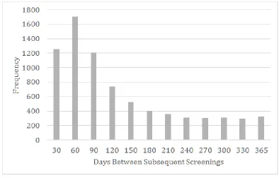
distribution of the duration between the FIT/FOBT and the colonoscopy, (Figure 2.7).

Figure 2.7Histogram of time between FIT/FOBT and subsequent colonoscopy

(32)

place within 6 months of a FIT/FOBT screening as diagnostic. Because going through a diagnostic

procedure (regardless of outcome) is likely to alter screening behavior following the colonoscopy,

we opt to eliminate individuals (n=5,690) who are identified as receiving a diagnostic colonoscopy

as a follow-up after a FIT/FOBT. Therefore, the final claims dataset for this dissertation work is

comprised of 181,012 individuals who are associated with 136,131 CRC screening claims.

2.2.3 Data Adjustments

Among the remaining data, 3,702 individuals have multiple CRC screenings within the same calendar

year. In order to aggregate screening behavior trajectory to an annual decision epoch, we preserve

the first CRC screening claim in the calendar year and eliminate subsequent screenings that occur

in the same calendar year. This does not impact the number of individuals captured by the dataset,

but does eliminate 4,188 screening records.

Additionally, the claims data contain a handful of screenings which occur borderline to our

observation period. These are screenings which occur on the last few days of 2009, or the first few

days of 2015, and are likely a result of the random toggle which is applied to the service date in order

to ensure patient anonymity. In order to capture these screenings while maintaining a consistent

observation window, we designate these screenings as occurring in 2010 and 2014 respectively.

2.2.4 Demographic Statistics

The data exclusions and criteria are diagrammed in Figure 2.1, and we compare the demographic

distribution of the dataset before and after exclusions are made in Table 2.3.

The most significant difference is the population distribution across the strata after exclusions

are made appears to be an increase in the proportion of individuals living in urban communities.

This shift occurs when we exclude those who are only partially observed in the dataset over the 5 year

interval. We speculate that the rural population may be more transient with respect to insurance

(33)

Table 2.3Demographic Comparison of Commercial Population Before and After Exclusions

After Exclusion (Counts) Before Exclusions (Counts)

Urban Rural Totals Urban Rural Totals

Male 32.7% 14.8% 47.5% 31.5% 16.6% 48.2%

Female 36.5% 16.0% 52.5% 34.0% 17.8% 51.8%

Totals 69.2% 30.8% 65.6% 34.4%

Male (59,168) (26,811) (85,979) (210,024) (110,654) (320,678)

Female (66,159) (28,910) (95,069) (226,380) (118,659) (345,039)

Totals (125,327) (55,721) (436,404) (229,313)

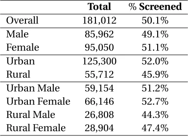
2.2.5 Screening Statistics

Descriptive statistics of screening prevalence is shown in Table 2.4 by subpopulation. We see that

women typically screen at slightly higher rates than men (51.1% vs 49.1%), and that individuals

living in urban metropolitan areas are significantly more likely to to screen in comparison to the

rural population (52% vs 45.9% respectively).

Table 2.4Statistics of screening prevalence is shown by subpopulation

Total %Screened

Overall 181,012 50.1%

Male 85,962 49.1%

Female 95,050 51.1%

Urban 125,300 52.0%

Rural 55,712 45.9%

Urban Male 59,154 51.2%

Urban Female 66,146 52.7%

Rural Male 26,808 44.3%

Rural Female 28,904 47.4%

Of individuals that make CRC screening claims within our 5 year observation window,

signifi-cantly more receive colonoscopies compared to FIT/FOBT screenings (64.7% vs 44.4%) (Table 2.5).

This difference is more pronounced in rural populations, especially among rural females. Despite

(34)

Table 2.5Screening statistics by subpopulation. FIT/FOBT and Colonoscopy statistics denote the portion of the population who received a FIT/FOBT or a Colonoscopy within the 5 year observation time

Ever Screened Colonoscopy First FIT/FOBT Colonoscopy Dual

Overall 90,769 58.6% 44.3% 64.7% 9.0%

Male 42,183 60.9% 41.9% 66.3% 8.2%

Female 48,586 56.6% 46.5% 63.2% 9.7%

Urban 65,166 56.8% 46.0% 62.8% 8.9%

Rural 25,603 63.1% 40.0% 69.3% 9.3%

Urban Male 30,298 58.7% 44.1% 64.2% 8.3%

Urban Female 34,868 55.2% 47.7% 61.7% 9.4%

Rural Male 11,885 66.6% 36.2% 71.9% 8.1%

Rural Female 13,718 60.1% 43.3% 67.0% 10.3%

have screening claims within the 5 year observation period receive both colonoscopy and FIT/FOBT

screenings. This occurs at higher rates for women as compared to men, particularly in rural areas.

Figure 2.8 shows the observed incidence rates of screening by age cohort. Although not extreme,

we do observe that cohorts who are observed around age 50 and 60 are more likely to have a

colonoscopy screening than other individuals. In contrast, the prevalence of FIT/FOBT screening

appears roughly consistent across ages.

(35)

These claims data are used to inform modeling strategies for CRC screening behaviors as detailed

in Chapters 2-5. It is important to note that observed insurance claims do not necessarily offer

a comprehensive understanding of screening behavior. However, we use the claims data which

indicates a receipt of screening as a basis to speculate about aspects screening behaviors such as

(36)

CHAPTER

3

STATISTICAL CLASSIFICATION OF

SCREENING BEHAVIOR

Statistical classification models are commonly used to model agent choice among a set of discrete,

mutually exclusive options. These models are a type of discrete choice methodology frequently used

in economic analyses to describe the causal relationship between the agent (and its characteristics)

and the choice out of the set of options (and their characteristics)[McFadden, 1973; Train, 2009].

These typically use data obtained from stated preference experiments or surveys which are designed

to efficiently elicit individual preference and enable the analysis of the driving forces behind these

preferences[Sanko, 2001]. These models are widely used in market research[Akinci et al., 2007]and

transportation demand modeling[Murat & Uludag, 2008].

In simulation models, statistical classification has been used as inputs to capture heterogeneous

(37)

[Waddell, 2000]to the decision to leave an emergency department waiting room[Hoot et al., 2008],

or predicting individual smoking behavior[Smith et al., 2011]. Most similar to the context of CRC

screening, logistic regression has been used to predict mammography noncompliance[Gierisch

et al., 2010], which has been implemented in a discrete event simulation and system dynamics

hybrid model of breast cancer screening policy analysis[Tejada et al., 2014].

An advantage to using statistically driven choice models is that they can provide nuanced insights

into causal relationships which can inform intervention strategies and provide a basis for predicting

response to changes in the choice set.

In this chapter we explore the use of statistical classification approaches to modeling CRC

screening choices and behaviors, first using binary classifiers (in Section 3.1), and then using

multiclass classifiers (Section 3.2). The performance of these models as classifiers are discussed

in each section, while their performance in generating representative trajectories is discussed in

Section 3.3.

3.1

Sequential Binary Classification

In the current implementation of the NC-CRC microsimulation model[Lich et al., 2017]screening

behavior is modeled using two binary classification models in sequence. Screening behavior is

assumed to be governed by two separate decision components: a choice regarding compliance (to

screen or not to screen), and a choice regarding modality (colonoscopy or FIT/FOBT). Both of these

are modeled using logistic regressions.

3.1.1 Methods

The probability of compliance is estimated based on individual characteristics (in our data: gender

and geography) using a logistic regression. A subset of the claims data is used in which individuals

are observed for the full 5 year window, beginning at age 50. This age specific subset is chosen as it

best captures organic screening behavior as screenings observed during these ages can reasonably

(38)

For the commercially insured this data subset is made up of 15,630 individuals.

The 5 year probability of screening compliance for an individual j,P5,j is estimated using the

logistic regression equation shown in 3.1

LetX_j =

 



1 if patient j is screened between ages 50 and 54

0 otherwise

(3.1)

P5j =E[Xj] =

exp(β0+β1Genderj +β2Geographyj)

1+exp(β0+β1Genderj+β2Geographyj)

(3.2)

To predict modality we assume that each individual is inherently either a colonoscopy screener,

or a FIT/FOBT screener. We estimate the probability that an individual is a colonoscopy screener

using a logistic regression, as shown in Equation 3.3. This logistic regression model is informed by

the subset of claims data in which individuals are observed for the full 5 year window, beginning at

age 50 (in order to capture what can reasonably be assumed to be the first screening choice), who

took part in some screening modality within the time period. For the commercially insured, this

subset of data is comprised of 9,092 individuals. For each individual in this subset, the response

variable is whether or not the individual’s first screening is a colonoscopy.

Pr(Modality is Colonoscopy|Gender, Geography)

= exp(β0+β1Gender+β2Geography)

1+exp(β0+β1Gender+β2Geography)

(3.3)

3.1.2 Results

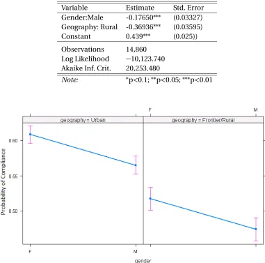
Table 3.1 shows the parameter estimation for this regression model, and Figure 3.1 shows effects

plots and the computed probabilities of screening by gender and geography, as well as the 95%

(39)

Table 3.1Logistic regression estimates to predict the probability of compliance (receiving a screen of any kind) for individuals observed for ages 50-54

Variable Estimate Std. Error

Gender:Male -0.17650∗∗∗ (0.03327)

Geography: Rural -0.36936∗∗∗ (0.03595)

Constant 0.439∗∗∗ (0.025))

Observations 14,860

Log Likelihood −10,123.740

Akaike Inf. Crit. 20,253.480

Note: ∗p<0.1;∗∗p<0.05;∗∗∗p<0.01

(40)

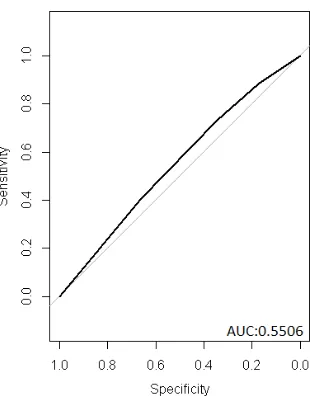
Figure 3.2ROC for compliance prediction model

The estimated parameters of the modality logistic regression are shown in Table 3.2. Figure 3.3

shows the computed probabilities of colonoscopy as a preferred modality by gender and geography

as well as the 95% confidence bounds associated with each estimate, and Figure 3.4 shows the ROC

curve.

Table 3.2Logistic regression estimates to calculate the probability that an individual receives a colonoscopy as their first screen, for individuals observed between ages 50-54

Variable Estimate Std. Error

Gender:Male 0.24242∗∗∗ (0.04619)

Geography: Rural 0.23859∗∗∗ (0.05251)

Constant 0.39628∗∗∗ (0.03320))

Observations 8,331

Log Likelihood −5,431.520

Akaike Inf. Crit. 10,869

(41)

Figure 3.3Effects plot for modality logistic regression

Figure 3.4ROC Curve for Modality Prediction Model

(42)

demographics. The screening compliance model indicates that males and rural individuals are less

likely to comply with screening recommendations in the first five years of their screening eligibility.

The modality prediction model indicates that when males and rural individuals do screen, they are

more likely to screen via colonoscopy instead of FIT/FOBT.

3.1.3 Simulation Implementation

For implementation as a behavior model in a simulation, the five year compliance probability can

be adjusted to an n-year probability dependent on the compliance decision epoch (which may be

modality specific) under an assumption of the binomial distribution, as detailed in Equation 3.4.

Pr(Screen in n years|Screen in 5 years w.p.P₅) =1−(1−P₅)n/5 (3.4)

Implicit in this approach is the assumption that the random variableXj is independent and

identically distributed (iid). In other words, it is assumed that for any given patient, the screening

probability is uniformly distributed with respect to time regardless of the screening decision epoch.

This assumption is necessary for this modeling approach, though it presents a notable limitation.

The two logistic regression models are implemented in sequence in the simulation model. As

shown in Figure 3.5, an individual’s modality choice is predicted (and fixed) using the modality

logistic regression, followed by repeated decisions about compliance, predicted by the

compli-ance logistic regression. Note that a critical assumption is that the probability of complicompli-ance is

independent of screening modality. This approach is based on a current implementation of the

NC-CRC model[Lich et al., 2017], and acts as a performance benchmark for predicting screening

behavior. In the model implementation, more dependent variables are incorporated (such as county

characteristics, distance to endoscopy center, etc), as the logistic regressions are based on a dataset

which contains richer location data. For the purposes of this analysis, we opt to apply the same

approach (albeit stripped of location specific characteristics) to the Oregon dataset in order to

(43)

Figure 3.5Choice structure for the sequential logistic regression modeling approach

3.2

Multiclass Classification

In the previous section, CRC screening behaviors are modeled as the result of two components

of choice: first modality (which then became fixed), and then compliance. In this section, choice

is modeled as a single choice between three behavior outcomes. In every routine screening year

an individual has the choice between non-compliance and screening with either a FIT/FOBT or

Colonoscopy (Figure 3.6). Non-compliance essentially becomes a modality within the model in any

given year. In this structure, an individual’s modality can change over their lifetime.

Multiclass classification is a generalization of binary classification which modifies binary

clas-sification algorithms to apply to cases where it is necessary to classify instances into 3 or more

classes.

Under this choice structure, we classify the data into 3 mutually exclusive outcomes:

• No screen is observed in the 5 year window

• A CRC screening is observed in the 5 year window, and the first observed screening is FIT/FOBT

• A CRC screening is observed in the 5 year window, and the first observed screening is a

(44)

Figure 3.6Choice structure for the multinomial logistic regression modeling approach

3.2.1 Methods

The most common multiclass classification algorithm is the multinomial logistic regression which

generalizes the binary logistic regression previously described in this chapter. The multinomial

logistic regression is often used to model choice, and in this context the primary assumption is

the independence of irrelevant alternatives (IIA). The assumption states that the relative odds of

preferring one outcome over another is unaffected by the presence of an additional alternative[Luce,

1959]. Whether or not the IIA assumption holds on a given dataset is most commonly evaluated

using the Hausman-McFadden test[McFadden, 1984], an approximate likelihood ratio test which

compares the estimates of a model fitted on a full set of alternatives to a model fitted on a specified

subset of alternatives.

In the case of the CRC claims data, the Hausman-McFadden test fails to validate the IIA

assump-tion. However, recent studies[Cheng & Long, 2007; Long & Freese, 2006]question the suitability of

such a test in applied contexts, and the literature demonstrates several instances[Belasco, 2013;

John & Thomsen, 2014; Kortesoja, 2009; Marinho & Mendes, 2013; Pulina, 2011; Ritter & Vance, 2013]

of multinomial logistic regression models that offer important insights despite an unvalidated (or

(45)

compute the screening outcome probabilities as:

Y_i=

            

N if if patient i is not screened between ages 50 and 54,

F 2 if the patient i is screened between ages 50 and 54, and screens FIT/FOBT,

C 3 if the patient i is screened between ages 50 and 54, and screens Colonoscopy

(3.5)

P r(Yi=k) =

eβk·Xi

P

l∈N,F,C eβl·Xi

(3.6)

When the IIA assumption does not hold, it is often standard practice to turn to the multinomial

probit model which relaxes this assumption by allowing the error terms in the utility function to

be correlated. Here we emulate existing empirical studies[Cheng et al., 2012; Comunian & Jewell,

2018; Dahl & Sorenson, 2010; Ehrmann & Tzamourani, 2012]which test the appropriateness of

their multinomial logistic regression model specification by fitting a probit model in parallel and

comparing the outcomes. Similar results indicate robust estimates.

Instead of using the logit link function in the logistic regression, a probit regression uses an

inverse normal link function. For a 3 case multiclassification problem, the probability of choosing

choice C under a probit model is

P r(Y_i=C) =P r("_{i N}−"i C<Vi C−Vi N,"i F−"i C<Vi C−Vi F) =

Z Vi C−Vi N+"i C

−∞

Z Vi C−Vi F+"i C

−∞

Z ∞

−∞

g("i C,"i F,"i N)d"i Cd"i Fd"i N

(3.7)

whereVi j represents the deterministic component of the utility of choice j for individuali,

g("i C,"i F,"i N)is the joint probability density function of the error terms"i N,"i C and"i F [Train,

2009]. The multinomial probit model has no closed form solution, so simulation is used to estimate

the model coefficients and predicted probabilities. The probit model is fit using the R package

MNP (version 3.1-0), which fits a Bayesian multinomial probit model using Markov chain Monte

(46)

developed by Imai and van Dyk[Imai & Van Dyk, 2005].

3.2.2 Results

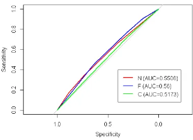
The estimated parameters for the multinomial logit model are shown in Table 3.3, and Figure 3.7

shows the computed probabilities (and strata effects) associated with each of the three possible 5 year

outcomes, for each of the 4 subpopulations. The ROC curves are shown in Figute 3.8. Similar to results

seen in Section 3.1, the multinomial model results indicate that both gender and geography are

significant predictors of screening outcomes for the first 5 years of screening eligibility. Individuals

living in urban areas more likely to screen FIT/FOBT over colonoscopy, and less likely to have no

CRC screenings in that time period. Additionally, males are less likely to screen FIT/FOBT over

colonoscopy, and more likely to not screen at all when compared to females.

Table 3.3Estimated parameters for the multinomial logit model

C F

Gender:Male −0.091∗∗ −0.331∗∗∗

(0.037) (0.045)

Geography:Rural −0.287∗∗∗ −0.523∗∗∗

(0.040) (0.050)

Constant −0.073∗∗ −0.471∗∗∗

(0.028) (0.032)

Akaike Inf. Crit. 31,123.040 31,123.040

(47)

Figure 3.7Effects plots for multinomial logistic regression

(48)

The mean parameters for the probit model are shown in Table 3.4. Estimation results are based

on a simulated chain where the first 150,000 samples are discarded as a burn-in period, followed

by 50,000 iterations. The results are consistent with those found in the multinomial logit model,

with those living in urban areas being less likely to have no screenings during the first 5 years of

screening eligibility, and with males being more likely to not screen when compared to females.

Table 3.4Mean multinomial probit parameter estimates (default choice is No Screen)

Choice Mean SD 95% confidence

C

(Intercept): -0.22434 0.137 -0.48573 0

Gender:Male -0.0177 0.025 -0.07281 0.024184

Geography: Urban 0.08701 0.048 0.01419 0.181069

F

(Intercept): -1.02292 0.298 -1.45121 -0.406362

Gender:Male -0.2148 0.052 -0.31121 -0.109517

Geography: Urban 0.31216 0.072 0.16956 0.456533

To compute the predicted probability associated with each outcome, we draw a sample of the

parameters from the 50,000 iterations. We repeat this 100 times for each population subgroup to

obtain the mean predicted probability estimates across the 100 sample draws shown in Table 3.5.

Note that the resulting predicted probabilities are extremely similar between these two multiclass

classifiers, although the underlying methodologies are different.

Table 3.5Mean predicted probability estimates from probit model vs logit probabilities

Logit Probabilities Probit Probabilities

N C F N C F

Rural Female 0.484 0.337 0.179 0.491 0.331 0.178

Rural Male 0.525 0.335 0.140 0.531 0.331 0.138

Urban Female 0.392 0.364 0.244 0.395 0.362 0.243

(49)

3.2.3 Simulation Implementation

Similar to the conversion described in Section 3.2, since these are probabilities based on a 5 year

ob-servation period we convert them to annual probabilities under the assumption of the multinomial

distribution using the multinomial probability density function as shown in Equation XX

LetPN,PC, andPF denote the annual probability of no screening, colonoscopy, and FIT/FOBT

respectively. We denote n year probabilities (probability of the outcome over the course of ann

year observation window) to beP(N)n,P(C)n, andP(F)n. The probability of no screening being observed in n years is:

P(N)n= n! n!0!0!P

n NP

0

CP

0

F (3.8)

This simplifies to

PN=P(N)1_n/n (3.9)

To compute the remaining annualized probabilities, consider that the probability that a

screen-ing occurs in an n year observation window, and the first screenscreen-ing observed bescreen-ing a colonoscopy

can be treated as separate, independent events. That is

P(C)n=

Pr(Colonoscopy before FIT/FOBT | a screening occurred in n years)∗Pr(screening occurred)

=Pr(Colonoscopy before FIT/FOBT| a screening occurred in n years)∗(1−P(N)n)

(3.10)

Further, consider that the probability that a colonoscopy is observed prior to a FIT/FOBT is

(50)

occurs before event F is equal to

An Examination of Individual Sequential Behavior Modeling in the Context of Healthcare Simulation.

ABSTRACT

APPROVED BY:

BIOGRAPHY

ACKNOWLEDGEMENTS

TABLE OF CONTENTS

LIST OF TABLES . . . vi

Chapter 3 Statistical Classification of Screening Behavior . . . 24

Chapter 5 Survival Analysis Models of Screening Behavior . . . 54

Chapter 6 Comparative Analyses . . . 74

Chapter 7 Conclusions and Recommendations . . . 97

BIBLIOGRAPHY . . . 99

LIST OF FIGURES

CHAPTER

Health Behavior in Simulation Models

Colorectal Cancer

Current Practices in CRC Screening Models

Research Objectives

CHAPTER

Observation Data

2.1.1 Initial Exclusions

2.1.2 Demographic Statistics

2.1.3 Observation Statistics

Screening Data

2.2.1 Initial Screening Data Exclusions

2.2.2 Diagnostic Screening Exclusions

2.2.3 Data Adjustments

2.2.4 Demographic Statistics

After Exclusion (Counts) Before Exclusions (Counts)

Total %Screened

Ever Screened Colonoscopy First FIT/FOBT Colonoscopy Dual

CHAPTER

Sequential Binary Classification

3.1.1 Methods

3.1.2 Results

3.1.3 Simulation Implementation

Multiclass Classification

3.2.1 Methods

3.2.2 Results

3.2.3 Simulation Implementation