Linearity Measures for
MQ
Cryptography
Simona Samardjiska1,2 and Danilo Gligoroski1 Department of Telematics, NTNU, Trondheim, Norway,1
FCSE, UKIM, Skopje, Macedonia.2
[email protected],[email protected], [email protected]
Abstract. We propose a new general framework for the security of multivariate quadratic (MQ) schemes with respect to attacks that exploit the existence of linear subspaces. We adopt linearity measures that have been used traditionally to estimate the security of sym-metric cryptographic primitives, namely the nonlinearity measure for vectorial functions introduced by Nyberg at Eurocrypt ’92, and the (s, t)–linearity measure introduced recently by Boura and Canteaut at FSE’13. We redefine some properties ofMQ cryptosystems in terms of these known symmetric cryptography notions, and show that our new framework is a compact generalization of several known attacks inMQ cryptography against single field schemes. We use the framework to explain various pitfalls regarding the successfulness of these attacks. Finally, we argue that linearity can be used as a solid measure for the sus-ceptibility ofMQschemes to these attacks, and also as a necessary tool for prudent design practice inMQcryptography.
Keywords Strong (s, t)–linearity, (s, t)–linearity, MinRank, good keys, separation keys
1 Introduction
In the past two decades, as a result of the advancement in quantum algorithms, the crypto community showed increasing interest in algorithms that would be potentially secure in the post quantum world. One of the possible alternatives are multivariate quadratic (MQ) public key cryptosystems based on the NP-hard problem of solving quadratic polynomial systems of equations over finite fields.
Many differentMQschemes emerged over the years most of which fall into two main cate-gories - single field schemes including UOV (Unbalanced Oil and Vinegar) [1], Rainbow [2], TTM (Tame Transformation Method) [3], STS (Stepwise Triangular System) [4], MQQ-SIG (Multivariate Quadratic Quasigroups - Signature scheme) [5], TTS (Tame Transfor-mation Signatures) [6], EnTTS (Enhanced TTS) [7] and mixed field schemes including C∗ [8], SFLASH [9], HFE (Hidden Field Equation) [10], MultiHFE [11,12], QUARTZ [13]. Unfortunately, over the years, most of them have been successfully cryptanalysed [14,15,4,16,17]. Three major types of attacks have proven devastating forMQ cryptosys-tems:
ii. Equivalent Keys attacks – based on finding an equivalent key for the respective scheme. The concept was introduced by Wolf and Preneel [19], and later further developed by Thomae and Wolf [16] to the generalization of good keys. The attacks on TTM [14], STS [4,16], HFE and MultiHFE [15,17] can all be seen from this perspective.
iii. Differential attacks – based on specific invariants of the differential of a given public key, such as the dimension of the kernel, or some special symmetry. It was introduced by Fouque et al. in [20] to break the perturbed version of the C∗ scheme PMI [21], and later also used in [22,23,24,25].
Interestingly, the history of MQcryptography has witnessed cases where, despite the at-tempt to inoculate a scheme against some attack, the enhanced variant has fallen victim to the same type of attacks. Probably the most famous example is the SFLASH [9] sig-nature scheme, that was build using the minus modifier on the already broken C∗ [26], and selected by the NESSIE European Consortium [27] as one of the three recommended public key signature schemes. It was later broken by Duboiset al. in [24,25] using a sim-ilar differential technique as in the original attack on C∗. Another example is the case of Enhanced STS [28], which was designed to be resistant to rank attacks, that broke its predecessor STS. Even the authors themselves soon realized that this was not the case, and the enhanced variant is vulnerable to a HighRank attack.
Such examples indicate that the traditional “break and patch” practice in MQ cryptog-raphy should be replaced by a universal security framework. Indeed, in the last few years, several proposals have emerged that try to accomplish this [29,30,31]. Notably, the last two particularly concentrate on the properties of the differential of the used functions, a well known cryptanalytic technique from symmetric cryptography. We will show here that an-other well known measure from symmetric cryptography, namely linearity, is fundamental for the understanding of the security of MQschemes.
1.1 Our Contribution
We propose a new general framework for the security of MQ schemes with respect to attacks that exploit the existence of linear subspaces. Our framework is based on two linearity measures that we borrow from symmetric cryptography, and adopt them suitably in the context ofMQcryptography. To our knowledge, this is the first time that the notion of linearity has been used to analyse the security ofMQ schemes.
We devise two generic attacks that separate the linear subspaces, and that are a general-ization of the aforementioned known attacks. We present one of the possible modellings of the attacks using system solving techniques, although other techniques are possible as well. Using the properties of strong (s, t)–linearity and (s, t)–linearity, we show what are the best strategies for the attacks. Notably, the obtained systems of equations are equivalent to those that can be obtained using good keys [16], a technique based on equivalent keys and missing cross terms. By this we show that our new framework provides a different, elegant perspective on why good keys exist, and why they are so powerful in cryptanalysis. Furthermore, we use our framework to explain various pitfalls regarding design choices of MQ schemes and the successfulness of the linear attacks against them. Finally, we argue that linearity can be used as a solid measure for the susceptibility ofMQschemes to linear attacks, and also as a necessary tool for prudent design practice in MQcryptography.
1.2 Organization of the Paper
The paper is organized as follows. In Section 2 we briefly introduce the design principles of MQ schemes and also recall the well known measure of nonlinearity of functions. In the next Section 3, we introduce the notion of strong (s, t)–linearity, which is basically an extension of the standard linearity measure and review the recently introduced (s, t)– linearity measure. In Sections 4 and 5 we show how the two linearity measures fit in the context of MQ cryptography. Some discussion on the matter proceeds in Section 6, and the conclusions are presented in Section 7.
2 Preliminaries
Throughout the text, Fq will denote the finite field of q elements, where q = 2d, and
a= (a1, . . . , an)| will denote a vector fromFnq.
2.1 Vectorial Functions and Quadratic Forms
Definition 1. Let n, m be two positive integers. The functions from Fnq to Fmq are called (n, m) functions or vectorial functions. For an (n, m) function f = (f1, . . . , fm), fi are
called the coordinate functions of f.
Classically, a quadratic form
f(x1, . . . , xn) =
X
1≤i≤j≤n
γijxixj :Fnq →Fq
can be written as x|Fx using its matrix representation F. This matrix is constructed differently depending on the parity of the field characteristic. In odd characteristic, F is chosen to be a symmetric matrix, whereFij =γij/2 fori6=jandFij =γij fori=j. Over fieldsFqof even characteristicFcan not be chosen in this manner, since (γij+γji)xixj = 0 fori6=j. Instead, letFe be the uniquely defined upper-triangular representation off,i.e., e
Fij =γij for i≤j. Now, we obtain a symmetric form by F:=Fe+eF|. Note that, in this
2.2 MQ Cryptosystems
The public key of a MQ cryptosystem is usually given by an (n, m) function P(x) = (p1(x), . . . , pm(x)) :Fnq →Fmq , where
ps(x) =
X
1≤i≤j≤n
e
γij(s)xixj+ n
X
i=1
e
βi(s)xi+αe
(s)
for every 16s6m, and wherex= (x1, . . . , xn)|.
The public key P is obtained by masking a structured central (n, m) function F = (f1, . . . , fm) using two secret linear transformations S, T ∈GLn(Fq) and defined as P =
T ◦ F ◦S.We denote by P(s) and F(s) the (n×n) matrices describing the homogeneous quadratic part of ps and fs, respectively.
Example 1.
i. The internal map of UOV [1] is defined asF :Fnq →Fmq , with central polynomials
fs(x) =
X
i∈V,j∈V
γij(s)xixj+
X
i∈V,j∈O
γij(s)xixj+ n
X
i=1
βi(s)xi+α(s), (1)
for every s = 1. . . m, where n = v +m, V = {1, . . . , v} and O = {v+ 1, . . . , n} denote the index sets of the vinegar and oil variables, respectively. The public map P is obtained byP =F ◦S, since the affineT is not needed (Indeed, any component
w|· F has again the form 1).
ii. The internal mapF :F2n →F2n ofC∗ [8] is defined by
F(x) =x2`+1,where gcd(2`+ 1,2n−1) = 1.
This condition ensures thatF is bijective.
iii. The representatives of the family of Stepwise Triangular Systems (STS) [4] have an internal map F : Fnq → Fmq defined as follows. Let L be the number of layers, and let ri,0 ≤ i ≤ L be integers such that 0 = r0 < r1 < · · · < rL = n. The central polynomials in thek-th layer are defined by
fi(x1, . . . , xn) =fi(x1, . . . , xrk), rk−1+ 1≤i≤rk.
We describe briefly two important cryptanalytic tools in MQ cryptography, that are of particular interest for us.
The MinRank Problem The problem of finding a low rank linear combination of matrices is a known NP-hard linear algebra problem [34] known as MinRank in cryptog-raphy [18]. It has been shown that it underlies the security of severalMQ cryptographic schemes [14,4,15]. It is defined as follows.
MinRank M R(n, r, k, M1, . . . , Mk)
Input:n, r, k∈N, where M1, . . . , Mk∈ Mn×n(Fq).
Question: Find – if any – a k-tuple (λ1, . . . , λk)∈Fkq\ {(0,0, . . . ,0)}such that:
Rank k
X
i=1
λiMi
!
Good Keys The concept of equivalent keys formally introduced by Wolf and Preneel in [35] is fundamentally connected to the security of MQschemes. In essence, any key that preserves the structure of the secret map is an equivalent key. This natural notion was later generalized by Thomae and Wolf [16] to the concept of good keys that only preserve some of the structure of the secret map. Good keys improve the understanding of the level of applicability of MinRank against MQschemes, and are a powerful tool for cryptanalysis. Good keys are defined as follows.
Let k,1 ≤ k ≤ m and F = {f1, . . . , fm} be a set of polynomials of Fq[x1, . . . , xn]. Let
I(k) ⊆ {xixj|1 ≤ i ≤ j ≤ n} be a subset of the degree-2 monomials, and let F
I = {f1
I(1), . . . , fm
I(m)} wherefk
I(k) :=
P
xixj∈I(k)
γ(k)ij xixj.
Definition 2 ([16]). Let (F, S, T),(F0, S0, T0) ∈ Fq[x1, . . . , xn]m ×GLn(Fq)×GLm(Fq)
Let also J(k)(I(k) for allk,1≤k≤m with at least oneJ(k)6=∅. We call (F0, S0, T0)∈ Fq[x1, . . . , xn]m×GLn(Fq)×GLm(Fq) a good key of (F, S, T) if and only if:
T ◦ F ◦S=T0◦ F0◦S0∧F
J =F
0
J
.
2.3 Linearity of Vectorial Functions
Linearity is one the most important measures for the strength of an (n, m) function for use in symmetric cryptoprimitives. We provide here some well known results about this notion.
Definition 3 ([32]). The linearity of an (n, m) function f is measured using its Walsh transform, and is given by
L(f) = max w∈Fm
q \{0},u∈Fnq | X
x∈Fnq
(−1)w|·f(x)+u|·x|
The nonlinearity of an (n, m) function f is the Hamming distance between the set of nontrivial components w|·f|w∈Fmq \ {0} of f and the set of all affine functions. It is given by
N(f) = (q−1)(qn−1− 1
qL(f)).
Definition 4. A vector w∈Fn
q is called a linear structure of an (n, m) function f if the
derivative Dwf(x) =f(x+w)−f(x) is constant,i.e., if
f(x+w)−f(x) =f(w)−f(0)
for all x∈Fn
q. The space generated by the linear structures of f is called the linear space
of f.
Proposition 1 ([32]). The dimension of the linear space of an (n, m) function is invari-ant under bijective linear transformations of the input space and of the coordinates of the function.
Proposition 2 ([32]). Let x|Fx be the matrix representation of a quadratic form f. Then, the linear structures of f form the linear subspace Ker(F).
The linear structures can provide a measure for the distance of the quadratic forms from the set of linear forms. Indeed the link is given by the following theorem.
Theorem 1 ([32]).
1. Let x|Fx be the matrix representation of a quadratic form f, and let Rank(F) = r. Then the linearity off is L(f) =qn−r2.
2. Let f be a quadratic (n, m) function, and let x|Fwx denote the matrix
representa-tion of a component w| ·f. Then the linearity of f is L(f) = qn−r2, where r = min{Rank(Fw)|w∈Fm
q }.
It is well known that the linearity of an (n, m) function is bounded from below by the value L(f) > qn2, known as the covering radius bound. It is tight for every even n, and functions that reach the bound are known as bent functions. It is also known, from [36] that bent functions exist only for m 6 n/2. A class of quadratic bent functions that has been extensively studied in the literature is the class of Maiorana-McFarland bent functions [37]. In general, an (n, m) function from the Maiorana-McFarland class has the form f = (f1, f2, . . . , fm) :F2n/2×F2n/2 →Fm2 where each of the componentsfi is
fi(x, y) =L(πi(x)y) +gi(x), (2) whereπiare functions onF2n/2,Lis a linear function ontoFm2 andgiare arbitrary (n/2, m) functions. Nyberg [36] showed that f is an (n, m)-bent function if every nonzero linear combination of the functions πi, i∈ {1, . . . , m} is a permutation onF2n/2.
Since the minimum linearity (maximum nonlinearity) is achieved only for m 6n/2, per-mutations can not reach the covering radius bound. But, they can reach the Sidelnikov-Chabaud-Vaudenay (SCV) bound [38], valid for m≥n−1, which for m=nodd, can be stated as: L(f)>qn+12 . (n, n) functions, where nis odd, that reach the SCV bound with equality, are called Almost bent (AB) functions.
As a direct consequence of Theorem 1 and the aforementioned bounds we have that quadratic (n, m) functions are
i. bent if and only if Rank(Fw) =nfor everyw|·f,
ii. almost bent if and only if Rank(Fw) =n−1 for every w|·f.
3 Strong (s, t)–linearity and (s, t)–linearity
Definition 5. Let f be an (n, m) function. Then, f is said to be strongly (s, t)–linear if there exist two linear subspaces V ⊂ Fn
q, W ⊂Fmq with Dim(V) = s, Dim(W) = t such
that for all w∈W, V is a subspace of the linear space of w|·f.
Compared to the standard measure for linearity given in Definition 3, that actually mea-sures the size of the vector space V, strong (s, t)–linearity also measures the size of the vector space W. We will see that this is particularly important in the case of MQ cryp-tosystems. We next provide some basic properties about strong (s, t)–linearity.
Proposition 3. If a function is strongly (s, t)–linear, then it is also strongly (s−1, t)– linear, and strongly (s, t−1)–linear.
Proposition 4. Let f be an quadratic (n, m) function and V ⊂ Fnq and W ⊂ Fmq with Dim(V) =s,Dim(W) =tbe two linear spaces. Thenf is strongly(s, t)–linear with respect to V, W if and only if the function fW corresponding to all components w|·f,w∈W can
be written as
fW(x, y) =gW(x) +LW(y)
where Fnq is the direct sum of U andV, gW is a quadratic function from U toFtq and LW
is a linear function from V toFtq.
Proof. From Definition 5,f is strongly (s, t)–linear with respect toV, W if and only ifV
is a subspace of the linear space ofw|·f, for allw∈W. Now, for wa basis vector ofW,
w|·f can be written as w|·f(x, y) = gw(x) +Lw(y) where y ∈V belongs to the linear space ofw|·f. Combining all the components for a basis ofW we obtain the desired form.
Proposition 5. Let f be a quadratic (n, m) function. Then f is strongly (s, t)–linear with respect to V, W if and only if the functionfW corresponding to all componentsw|·f,
w∈W is such that all its derivatives Daw|·f, witha∈V are constant.
Recently, Boura and Canteaut [33] introduced a new measure for the propagation of linear relations through S-boxes, called (s, t)-linearity.
Definition 6 ([33]). Let f be an (n, m) function. Then, f is said to be (s, t)–linear if there exist two linear subspaces V ⊂ Fnq, W ⊂Fqm with Dim(V) = s, Dim(W) = t such
that for all w∈W, w|·f has degree at most 1 on all cosets of V.
Similarly as for strong (s, t)–linearity, it is true that
Proposition 6 ([33]). If a function is (s, t)–linear, then it is also (s−1, t)–linear, and
(s, t−1)–linear.
Boura and Canteaut [33] proved that any (s, t)–linear function “contains” a function of the Maiorana-McFarland class, in the following sense.
V, W if and only if the function fW corresponding to all components w|·f, w ∈W can
be written as
fW =M(x)·y+G(x)
where Fnq is the direct sum of U andV, Gis a function from U toFtq andM(x)is a t×s
matrix whose coefficients are functions defined on U.
A useful characterization of (s, t)–linearity, resulting from the properties of the Maiorana-McFarland class is through second order derivatives defined byDa,bf =DaDbf =DbDaf.
Proposition 8 ([33]). Let f be an (n, m) function. Then f is (s, t)–linear with respect to V, W if and only if the functionfW corresponding to all components w|·f, w∈W is
such that all its second order derivatives Da,bw|·f, with a, b∈V vanish.
The two measures of linearity, even though they measure different linear subspaces are also interconnected. The following two propositions illustrate this connection.
Proposition 9. If a function is strongly (s, t)–linear, then it is also (s, t)–linear.
Proposition 10. If a quadratic(n, m) functionf is(dn2e+s,1)–linear than it is strongly
(2s,1)–linear.
Proof. From Proposition3 [33] we have the fact that a (s,1)–linear function has linearity L(f)>qs (This comes from the fact that the linearity of a function is lower bounded by the linearity of any of its components.) Thus, if a quadratic (n, m) function is (dn2e+s,1)– linear, then L(f)>qdn2e+s. From Theorem1L(f) =qn−
r
2, wherer = min{Rank(Fw)|w∈ Fmq }. From heren−r2 >d
n
2e+sand furthern−2s>r. Hencef is strongly (2s,1)–linear. In the next two sections we will provide a general framework for the security of MQ schemes against linear cryptanalysis using the notions of strong (s, t)–linearity and (s, t)– linearity.
4 The strong (s, t)–linearity measure for MQ systems
In this section, we show that strong (s, t)–linearity is fundamentally connected to the susceptibility of an MQ scheme to MinRank attacks and good keys attacks.
From Proposition 2 we have the following theorem.
Theorem 2. Letf = (f1, f2, . . . , fm)be a quadratic(n, m)function, and letF1,F2, . . . ,Fm
be the matrix representations of the coordinates of f.
Then the MinRank problem M R(n, r, m,F1,F2, . . . ,Fm) has a solution if and only if f is strongly (n−r,1)–linear.
Proof. We can see thatv = (v1, . . . , vn)∈Fnq\ {0}is a solution to the MinRank problem
M R(n, r, m,F1,F2, . . . ,Fm) if and only if
Rank n
X
i=1
viFi
!
that is, if and only if Dim Ker n
X
i=1
viFi
!!
>n−r,i.e.,from Proposition 2, if and only ifv|·f has at leastn−rlinearly independent linear structures. TakingW to be the space generated by the vectorv andV to be the linear space ofv|·f, from Definition 5 the last is equivalent to f being strongly (n−r,1)–linear.
Example 2. From Theorem 2 it is clear that bent functions are resistant to MinRank attacks, since no linear combination of the components of the function has smaller rank than n. Thus, regarding MinRank attacks, bent functions are optimal for use as a secret map in MQcryptosystems.
Example 3. Regarding encryption MQ schemes, a natural conclusion would be that AB permutations are the most suitable for use. One of the most scrutinized AB permutations are the Gold functions defined over Fqn for oddn by:
f(x) =xq`+1, gcd(q`+ 1, qn−1) = 1, gcd(`, n) = 1
where the first condition guarantees balancedness, and the second AB-ness. Notably, one of the most famous MQ schemes, the C∗ scheme, uses an AB function, although there are variants that do not meet the second condition [21].
As mentioned before, AB functions have Rank(Fv) = n−1 for any component v|·f. This means that each of the components have a linear space of dimension 1, and no two components share a linear space, i.e.,AB functions are only strongly (1,1)–linear. Hence, MinRank for r=n−1 is trivially satisfied and does not reveal anything more about the structure of the map.
The example of Gold functions from Example 3 implies that although MinRank on its own can be a good indicator of a weakness in a scheme, it does not provide a sufficient condition for mounting a successful attack. A better framework for the applicability of MinRank is provided by the concept of good keys (cf. Section2.2). It should be emphasized that the definition of good keys (Definition 2), does not explicitly state the structure that is being preserved, thus, providing a framework even for structures not yet discovered. On the other hand, the motivation for good keys comes from the Rainbow band separation attack [39], that exploits (among others) a particular weakness connected to the presence of linear structures in the secret map. Moreover, known attacks that use MinRank, as well as other applications of good keys, again take advantage of the same property. Hence, we give a new definition for the special type of keys that separate the space of linear structures. This definition comes as a direct consequence of strong (s, t)–linearity. Later, we will also take a look at another weakness that the Rainbow band separation attack and its generalizations take advantage of, and we will also define the corresponding keys. We will call both types of keys separation keys.
Definition 7. Let (F, S, T),(F0, S0, T0) ∈Fq[x1, . . . , xn]m×GLn(Fq)×GLm(Fq) and let P =T◦ F ◦S=T0◦ F0◦S0. We call(F0, S0, T0) a strong (s, t) separation keyfor P ifP is strongly (s, t)–linear with respect to two spaces V and W, Dim(V) =s, Dim(W) =tand
S0 =SV|, T0 =TW.
A strong (s, t) separation key separates the components of the public key that have a non empty common linear space. As a direct consequence of Definition 7 we have that:
Proposition 11. If (F0, S0, T0) is a strong (s, t) separation key for P, then it is also a good key for P.
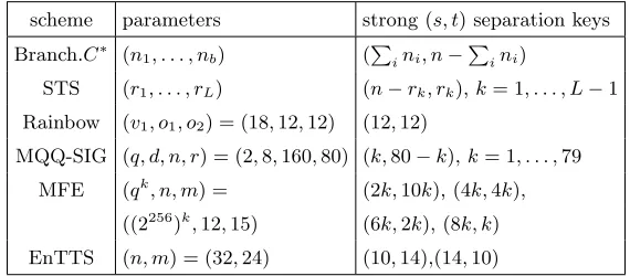
Many MQ cryptosystems, proposed so far have strong separation keys. As mentioned before, Rainbow [2] is one of the examples, but also all STS cryptosystems ([3,4]), and all MQcryptosystem that combine a layered structure with other types of design principles, including among others BranchedC∗ [40], MQQ-SIG [5], TTS [6], EnTTS [7], MFE [41]. Table 1 summarizes the different strong separation keys for some of these schemes.
Table 1.Examples of strong (s, t) separation keys for someMQcryptosystems
scheme parameters strong (s, t) separation keys Branch.C∗ (n1, . . . , nb) (Pini, n−Pini)
STS (r1, . . . , rL) (n−rk, rk),k= 1, . . . , L−1 Rainbow (v1, o1, o2) = (18,12,12) (12,12)
MQQ-SIG (q, d, n, r) = (2,8,160,80) (k,80−k),k= 1, . . . ,79 MFE (qk, n, m) = (2k,10k), (4k,4k),
((2256)k,12,15) (6k,2k), (8k, k) EnTTS (n, m) = (32,24) (10,14),(14,10)
The known attacks on these systems, can all be considered as separation key attacks involving different techniques and optimizations. The framework of strong (s, t) linearity provides a unified way of looking at these attacks, and a single measure that can be used as criteria for the parameters of schemes that have strong separation keys. The next two theorems explain in detail how to mount a generic strong separation key attack, what is the complexity of the attack, and what is the best strategy for attack when the existence of a strong separation key is known. We decided to present the attack by representing the conditions for strong (s, t) linearity as systems of equations. In this way we obtain completely equivalent systems to the ones that can be obtained using good keys, thus, offering another elegant point of view on why good keys exist. Note that this is not the only technique that can be used to recover strong (s, t) separation keys (for example we can use probabilistic approach). However, it provides a clear picture of the cases when the existence of a particular strong separation key is devastating for the security of MQ schemes.
Theorem 3. Let it be known that a strong (s, t) separation key exists for a given MQ
i. The task of finding a strong (s, t) separation key(SV|, TW) is equivalent to solving the
system of bilinear equations
Pw(i)·a(j)= 0, i∈ {1, . . . , t}, j ∈ {1, . . . , s}, (3)
in the unknown basis vectors w(i) of the spaceW, and the unknown basis vectorsa(j)
of the space V.
ii. The complexity of recovering the strong (s, t) separation key through solving the sys-tem (3)is
O
t·s·n·
(n−s)s+ (m−t)t+dreg
dreg
ω
(4)
wheredreg = min{(n−s)s+(m−t)t}+1, and26ω63is the linear algebra constant.
Proof. i. From Definition7 the existence of a strong (s, t) separation key (SV|, TW) means that P is strongly (s, t)–linear with respect to two spaces V, W of dimension Dim(V) =
s,Dim(W) = t. So the task is to recover these two spaces, i.e., to recover some bases {a(1), . . . , a(s)}and{w(1), . . . , w(t)}ofV andW respectively. From Definition 5 and Propo-sition 2, w ∈ W and a ∈ V if and only if a is in the kernel of Pw, i.e., if and only if
Pw·a= 0. Let the coordinates of the basis vectors {a(1), . . . , a(s)}and {w(1), . . . , w(t)}be unknowns. In order to insure that they are linearly independent, we fix the last s coordi-nates of a(j) to 0 except the (n−j+ 1)-th coordinate that we fix to 1, and similarly we fix the firsttcoordinates ofw(i)to 0 except thei-th coordinate that we fix to 1. In this way we can form the bilinear system (3). The solution of the system will yield the unknown bases of U and W. Note that if we get more than one solution, any of the obtained solutions will suffice. However, it can also happen that the system has no solutions. This is due to the fixed coordinates in the basis vectors, which can be done in the particular manner with probability of approximately (1− 1
q−1)
2. Still, if no solutions, we can randomize the function P by applying linear transformation to the input space and the coordinates of the function, since from Prop 1, this preserves the strong (s, t)–linearity of P.
ii. From i., the system (3) consists of t·s·n bilinear equations in two sets of variables of sizes ν1 = (n−s)s and ν2 = (m−t)t, bilinear with respect to each other. The best known estimate of the complexity of solving a random system of bilinear equations is due to Faugereet al. [42], which says that for the grevlex ordering, the degree of regularity of a generic affine bilinear zero-dimensional system over a finite field is upper bounded by
dreg≤min(ν1, ν2) + 1. (5)
Now, we use the F5 algorithm for computing a grevlex Gr¨obner basis of a polynomial system [43,44], that has a complexity of
O
µ·
ν1+ν2+dreg
dreg
ω
, (6)
for solving a system ofν1+ν2 variables andµ equations (26ω63 is the linear algebra constant). Using (5) and (6), we obtain the complexity given in (4).
Theorem 4. Let it be known that a strong (s, t) separation key exists for a given MQ
public key P :Fnq →Fqm with matrix representationsPw of a component w|· P.
i. The task of finding a strong(s, t) separation key can be reduced to 1. Solving the system of bilinear equations
P(i)w ·a(j)= 0, i∈ {1, . . . , c1}, j∈ {1, . . . , c2}, (7)
in the unknown basis vectors w(i) of the space W, and the unknown basis vectors
a(j) of the space V, where c!, c2 are small integers chosen appropriately.
2. Solving the system of linear equations
P(i)w ·a(j)= 0, i∈ {c1+ 1, ..., t}, j∈ {1, ..., c2},
P(i)w ·a(j)= 0, i∈ {1, ..., c1}, j∈ {c2+ 1, ..., s}, (8)
in the unknown basis vectors w(i), i ∈ {c1 + 1, . . . , t} of the space W, and the
unknown basis vectors a(j), j∈ {c2+ 1, . . . , s} of the space V.
ii. The complexity of recovering the strong(s, t)separation key using the procedure from i. is
O
(n−s)c2+ (m−t)c1+dreg
dreg
ω
(9)
where dreg = min{(n−s)c2,(m−t)c1}.
Proof. i. The crucial observation that enables us to prove this part, is a consequence of Proposition 3. Recall that it states that strong (s, t)–linearity implies strong (s−1, t) and strong (s, t−1)–linearity. Even more, if P is strongly (s, t)–linear, with respect to
V = Span{a(1), . . . , a(s)}, W =Span{w(1), . . . , w(t)}, then it is strongly (s−1, t)–linear with respect to V1, W, whereV1⊂V, and strongly (s, t−1)–linear with respect toV, W1, where W1 ⊂ W. Hence, there exist two arrays of subspaces V ⊃ V1 ⊃ · · · ⊃ Vs−1 and
W ⊃ W1 ⊃ · · · ⊃ Wt−1, such that P is strongly (s−i, t−j)–linear with respect to
Vi =Span{a(1), . . . , a(s−i)},Wj =Span{w(1), . . . , w(t−j)}. Thus, we can first recover the bases of some spaces Vs−c2, Wt−c1, and then extend them to the bases of V, W. Again, similarly, as in the proof of Theorem 3, we take the coordinates of the basis vectors {a(1), . . . , a(s)} and {w(1), . . . , w(t)} of V and W to be the unknowns, and again fix the last s coordinates of a(j) to 0 except the (n−j+ 1)-th coordinate that we fix to 1, and fix the firsttcoordinates ofw(i)to 0 except thei-th coordinate that we fix to 1. Next, we pick two small constants c1 and c2, and form the bilinear system (7). Once the solution of this system is known, we can recover the rest of the bases vectors, by solving the linear system 8.
ii. The main complexity for the recovery of the key is in solving the system (7). Thus, proof for the complexity (9) is the same as for ii. Theorem 3. What is left, is to explain how the constants c1 and c2 are chosen. First of all, the system (7) consists of c1·c2·n equations in (n−s)c2+ (m−t)c1 variables. We choose the constantsc1 andc2 such that
c1·c2·n >(n−s)c2+ (m−t)c1. Second, since the complexity is mainly determined by the value dreg = min{(n−s)c2,(m−t)c1}, these constants have to be chosen such that this value is minimized. Note that in practice, for actual MQ schemes, we can usually pick
The most important implication of the last theorem is that when n−s or m− t is constant we have a polynomial time algorithm for recovering a strong (s, t) separation key. This immediately implies that for any MQscheme with this property we can recover in polynomial time a subspace on which the public key is linear.
Another implication is that it provides the best strategy of attacking an MQ scheme that possesses some strong (s, t) separation key. Indeed, since we need to minimize dreg, we simply look for the minimal m−t or minimal n−s s.t. there exists a strong (s, t) separation key.
Example 4. Consider a (n, n) public key function from the family of STS systems (cf. Example 1.iii). From Table 1, for the parameter set (r1, . . . , rL) we see that the scheme has a strong (n−r1, r1) separation key and also a strong (n−rL−1, rL−1) separation key. For the first key, n−s = r1 is small, so we can choose c2 = 1 and c1 such that
c1n > r1+ (n−r1)c1,i.e., we can choosec1 = 2. For the second key,n−t=n−rL−1 is small so we can choose c1 = 1 and c2 such thatc2n > rL−1c2+ (n−rL−1), i.e., we can choose c2= 2. Note that for smallqit is perfectly fine to choosec1 =c2 = 1 in both cases, since then at most q solutions for the strong keys will need to be tried out.
The level of nonlinearity of a given function can be used as sufficient condition for the nonexistence of a strong (s, t) separation key.
Theorem 5. An (n, m) function f of linearity L(f) 6 qn−r2 does not posses a strong (s, t) separation key fors > n−r.
Proof. From the linearity given, f does not have any component whose linear space has dimension bigger than n−r. Thus,f is not strongly (s, t)–linear fors > n−r, and does not have a corresponding strong (s, t) separation key.
As a direct consequence, we have the following:
Corollary 1.
1. If (F0, S0, T0) is a strong (s, t) separation key for C∗, then s61 and t61.
2. UOV using Maiorana-McFarland bent function does not posses a strong (s, t) separa-tion key for any s >0.
5 The (s, t)-Linearity Measure for MQ schemes
The size of the linear space of the components of an (n, m) quadratic function clearly provides a measure for the applicability of the function in MQsystems. Still, the notion of strong (s, t)–linearity can not provide a measure for the existence of all the linear subspaces on which the restriction of an (n, m) function is linear.
original Oil and Vinegar scheme. Furthermore, the existence of such spaces improves the attack against Rainbow, compared to an attack that only considers linear spaces of the components.
We will show next that (s, t)–linearity provides a characterization for such subspaces, and thus, provides an improved measure for the security ofMQ schemes.
Example 5. Let P : Fnq → Fmq be a UOV public mapping. In Section 4 we saw that the secret map of an UOV scheme belongs to the Maiorana-McFarland class. Thus, immedi-ately, from Proposition 7, we conclude that P is (m, m)–linear,i.e., P is linear on the oil space.
Now, similarly as in the previous section, we can define a special type of separation key, that separates the spaces with respect to which a function is (s, t)–linear.
Definition 8. Let (F, S, T),(F0, S0, T0) ∈Fq[x1, . . . , xn]m×GLn(Fq)×GLm(Fq) and let P = T ◦ F ◦S = T0◦ F0◦S0. We call (F0, S0, T0) an (s, t) separation key for P if P is
(s, t)–linear with respect to two spaces V and W, Dim(V) =s, Dim(W) =t and
S0 =SV|, T0 =TW.
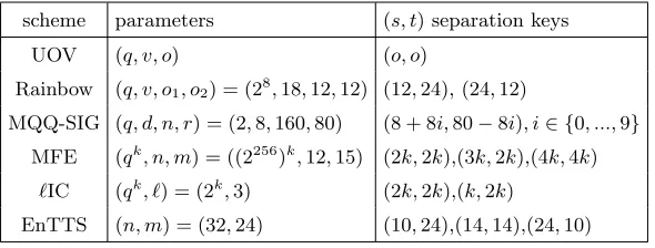
Conclusively, any public mapping that was created using an oil and vinegar mixing has a (s, t) separation key. Table 2 gives the (s, t) separation keys for some of theMQ schemes that combine a layered structure with oil and vinegar mixing.
Table 2.Examples of (s, t) separation keys for someMQcryptosystems
scheme parameters (s, t) separation keys UOV (q, v, o) (o, o)
Rainbow (q, v, o1, o2) = (28,18,12,12) (12,24), (24,12)
MQQ-SIG (q, d, n, r) = (2,8,160,80) (8 + 8i,80−8i), i∈ {0, ...,9}
MFE (qk, n, m) = ((2256)k,12,15) (2k,2k),(3k,2k),(4k,4k) `IC (qk, `) = (2k,3) (2k,2k),(k,2k)
EnTTS (n, m) = (32,24) (10,24),(14,14),(24,10)
An interesting case regarding (s, t)–linearity is the C∗ scheme for which we have the following result.
Proposition 12. Let F : Fn2 → Fn2 be the secret map of C∗ (cf. Example 1ii) and let gcd(`, n) =d. Then, there exists a (d, n) separation key for these parameters of C∗. Proof. First, let us consider the equationDa,x(f) = 0 for a nonzeroa. A little computation shows that it is equivalent to
and since we are interested in nonzero solutions we can restrict our attention to
a2`−1+x2`−1 = 0.
This equation has gcd(2`−1,2n−1) = 2d−1 independent roots (see for example [45]). Thus, there exists a space V of dimension Dim(V) = ds.t. Da,b(f) = 0, for all a, b ∈V. This implies that Da,b(w|·f) = 0, for any w ∈ Fn2. Further from Proposition 8 and Definition 8 it follows that there exists a (d, n) separation key for the given parameters. Hence, the best choice for parameters of the C∗ scheme is when d = 1, because in this case, the dimension of the space V is the smallest, and it is hardest to separate it. Note that this is analogous to the case of the UOV scheme, where also it is desirable to have smaller spaceV. The use of d >1 was exactly the property that was exploited by Dubois
et al. in [25] to break a modified version of the signature scheme SFLASH with d > 1 before the more secure version withd= 1 was broken due to the possibility to decompose the second order derivative into linear functions [24]. Even then the authors of [25] noted that the conditiond= 1 should be included in the requirements of the scheme, a fact that was overseen by the NESSIE consortium.
Note further that Proposition 12 implies that the dimension of the space V is invariant under restrictions of the public map (minus modifier). Thus, the SFLASH signature scheme also possesses a (d, k) separation key, where k 6 n is the number of coordinates of the public key of SFLASH, and can equivalently be used to attack the modified version. Similarly as for the case of strong (s, t) separation keys, (cf. Theorem 3 and Theorem 4), we can construct a generic algorithm that finds (s, t) separation keys. This part will be covered in the extended version of the paper. Here we focus our interest on a special type of separation keys, namely, (s, m) separation keys where the space W is the entire image space of the function. Indeed, schemes including UOV, Rainbow, Enhanced TTS, all posses exactly such keys. We will also show how the properties of (s, m)–linearity provide the best strategy for attacking schemes that posses (s, m) separation keys. Unfortunately, in this case it is more difficult to estimate the complexity of the attacks, since the obtained equations are of mixed nature. Therefore, we leave the complexity estimate for future work. Still, it is notable that we again arrive to equivalent systems of equation as in the case of good keys.
Theorem 6. Let it be known that an (s, m) separation key exists for a givenMQ public key P :Fnq → Fmq with matrix representations Pi := Pei+Pe|i of the coordinate functions
pi.
i. The task of finding an (s, m) separation key (SV|, TFm
q ) is equivalent to solving the
following system of equations
a(j)Pia(k)= 0, i∈ {1, ..., m}, j, k∈ {1, ..., s}, j < k
a(k)Peia(k)= 0, i∈ {1, ..., m}, k∈ {1, ..., s}, (10) in the unknown basis vectors a(j) of the space V.
1. First solving the system of equations
a(j)Pia(k)= 0, i∈ {1, ..., m}, j, k∈ {1, ..., c}, j < k
a(k)Peia(k)= 0, i∈ {1, ..., m}, k∈ {1, ..., c}, (11) in the unknown basis vectorsa(k),k∈ {1, . . . , c}of the spaceV, for an appropriately chosen integerc.
2. And then solving the system of linear equations
a(j)Pia(k)= 0, i∈ {1, ..., m}, j∈ {1, ..., c}, k∈ {c+ 1, ..., s}, j < k
in the unknown basis vectorsa(k), k∈ {c+ 1, ..., s} of the space V.
Proof. i. From Definition 8, P is (s, m)–linear with respect to V,Fmq where Dim(V) =
s. So we need to recover only some basis {a(1), . . . , a(s)} of V. From Definition 6 and Proposition 8, the condition for (s, t)–linearity can be written as Da(j),a(k)f = 0 for all
a(j), a(k) ∈ V, i.e., as a(j)P
ia(k) = 0. Since Da,af = 0 for any a, we must write this condition as a(k)Peia(k) = 0. We ensure the linear independence of the unknown basis
vectors{a(1), . . . , a(s)}by fixing the lastscoordinates ofa(j) to 0 except the (n−j+ 1)-th coordinate that we fix to 1. The probability that we can fix the coordinates of the basis vectors in this way is approximately 1−q−11. If the system does not yield a solution we randomize P. In this way we form the system (10). It consists of m s+12
equations in
s(n−s) variables.
ii. From Proposition 6, we have that if P is (s, m)–linear, with respect to a vector space
V = Span{a(1), . . . , a(s)}, Fmq , then it is (s−1, m)–linear with respect to V1,Fmq , where
V1 ⊂V. Hence, there exists an array of subspaces V ⊃ V1 ⊃ · · · ⊃ Vs−1, such that P is (s−i, m)–linear with respect to Vi = Span{a(1), . . . , a(s−i)}. Thus, we can first recover the basis of some space Vs−c and then extend it to the bases ofV. That is, we first solve (11), and then we are left with the linear system (12). What is left is how we choose the constantc. The system (11) consists ofm c+12 equations in (n−s)cvariables. It is enough to choose c such that m c+12 >(n−s)c, in order to get a unique solution for the basis vectors.
Remark 1. Conditions for (s, t)–linearity have been used in other attacks not involving good keys or system solving. For example, the analysis of UOV in [1] uses exactly the conditions of Proposition 8 in order to test whether a subspace is contained in the oil space. An equivalent condition is also used in [46] again for analysis of UOV, and the authors’ approach here is a purely heuristic one.
We conclude this part with an interesting result on the (s, m)–linearity of a random quadratic (n, m)-function.
Proposition 13. Let f be a randomly generated (n, m)-function over Fq. Then, we can
expect that there exist q
2(n−s)
m(s+1) different subspaces V, such that f is (s, m)–linear with
Proof. Let the (n, m)-function f be given. Then f is (s, m) linear with respect to some spaceV if and only if there existslinearly independent vectorsa(1), . . . , a(s)∈Fn
q such that
V =Span{a(1), . . . , a(s)} and f is linear on every coset ofV. Without loss of generality, we can fixscoordinates in each of thea(k)to ensure linear independence. In this manner, from the conditions of linearity from Theorem 6 we obtain a quadratic system of m s+12
equations ins(n−s) variables. We can expect that such a system, on average has around
q
s(n−s) m(s+12 ) =
q
2(n−s)
m(s+1) solutions. For simplicity, we assume that the coordinates can be fixed in the particular manner. (In general, this is possible with a probability of 1 − 1
q−1.) Note that all of these solutions span different subspaces. Indeed, suppose (a(1)1 , . . . , a(s)1 ) and (a(1)2 , . . . , a(s)2 ) are two different solutions. Then there exists i such that a(i)1 6= a(i)2 . Then a(i)2 is not in the span of a(1)1 , . . . , a(s)1 because the fixed coordinates ensure linear independence. Thus, all the solutions generate different subspaces.
Proposition 13 implies that random quadratic (n, m) functions most probably have an (b2n−m
m+2 c, m) separation key. For the case ofn=m, this means that there are no nontrivial (s, m) separation keys, but for the case of n= 2m, we can expect that there is a (2, m) separation key, and for n= 2m+ 4, even a (3, m) separation key.
Note that Proposition 13 further implies, that for n ≈ m2, a random quadratic (n, m) function is likely to have a (m, m) separation key. This is exactly the case identified by Kipnis et al. [1] as an insecure parameter set. See [1] for an efficient algorithm for recovering this space.
5.1 On the Reconciliation Attack on UOV
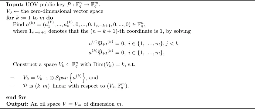
Recall the shape of the internal map of UOV from Example 1i. From Proposition7 and Proposition6 it follows that P is (i, m)–linear for any 1 6i 6 m. In order to break the scheme, it is necessary to find a vector space V, such thatP is (m, m)–linear with respect to (V,Fmq ). We will call any such space V an oil space. Ding et al. in [39] propose an algorithm that sequentially performs a change of basis that reveals gradually the space
V. They call the algorithm Reconciliation Attack on UOV. In Figure 1, we present an equivalent version of the attack interpreted in terms of (s, t)–linearity (cf. Algorithm 2 [39]).
It can be noticed that the Reconciliation attack is exactly an (s, m) separation key attack, where the constant c in Thm 6 is chosen to be c = 1. However, we will show that the choice of c= 1 is justified only for the (approximately) balanced version of UOV, and not for any parameter set.
For example, consider the UOV parameter set m= 28 andv= 56. The public key in this case has a (28,28) separation key. Using the reconciliation attack (equivalently if we take
Input:UOV public keyP:Fnq →Fmq . V0←the zero-dimensional vector space
fork:= 1 tomdo
Finda(k)= (a(k) 1 , ..., a
(k)
v ,0, ...,0,1n−k+1,0, ...,0)∈Fnq,
where 1n−k+1denotes that the (n−k+ 1)-th coordinate is 1, by solving a(j)Pia(k) = 0, i∈ {1, . . . , m}, j < k a(k)Peia(k) = 0, i∈ {1, . . . , m}, Construct a spaceVk⊂Fnq with Dim(Vk) =k, s.t.
– Vk=Vk−1⊕Span n
a(k)o, and
– Pis (k, m)–linear with respect to (Vk,Fmq).
end for
Output:An oil spaceV =Vmof dimensionm.
Fig. 1.Reconciliation Attack on UOV in terms of (s, t)–linearity
of 28 equations in 28 variables. In other words, this approach seems to work equally well for the balanced version of the scheme (when m=v) and for the unbalanced version. Now, consider a UOV public keyP :Fnq →Fmq . By definition it is (m, m)–linear, and also (s, m)–linear for everys6m. We can use Theorem 6 ii. to find the (m, m) separation key by choosingcsuch thatm c+12
>(n−m)c,i.e.,c >2(n/m−2). We suppose that we have fixed n−m coordinates of the vectors a(1), . . . , a(m) ∈Fn
q to ensure linear independence. Suppose instead that we have chosen c < 2(n/m −2). Then Step 1 of Theorem 6 ii. will give on average q2(n−m)/m(c+1) solutions for the basis vectors, and all the solutions span a different space of dimension c such that P is (c, m) linear with respect to it (cf. Proposition 13). From the choice of the basis vectors, only one of these spaces is a subspace of the oil space V we are trying to recover. Thus, if q2(n−m)/m(c+1) is relatively big, it is infeasible to find the correct subspace. If we choose a wrong space, after several steps (depending on n, m, c), we will not be able to find any new linearly independent vectors. The reason is that from Proposition 13 it is expected that even in the random case such subspaces exist, but their dimension is much smaller than that of the actual oil space. Hence, we must choose at least c ≈ 2(n/m−2). For example, c = 1 is suitable only for balanced versions where n ≈ 2m, c = 2 can be used for n upto ≈ 3m, and for the practically used parameters of 3m < n <4m cshould be 4 or even 5.
Remark 2. In [47], Thomae analyses the efficiency of the Reconciliation attack on UOV, and concludes that solving the equations from the first step of the attack is quite inefficient. He proposes instead to recover several columns from the good key at once and introduces some optimal parameter kfor the number of columns, that corresponds to our parameter
5.2 Combining strong (s, t)–linearity and (s, t)–linearity
A number of existingMQschemes combine several paradigms in their design. For example, Rainbow [2] or EnTTS [7] have a secret map with both layered and UOV structure. In other words, these schemes posses both types of separation keys. (Note that we do not talk about the trivial implication of a (s, t) separation key when a strong (s, t) separation key exists.) For example, Rainbow, with parameters (v, o1, o2), where n = v+o1 +o2,
m =o1+o2, has a (o2, o1+o2) separation key with respect to V,Fmq , but also a strong (o2, o1) separation key with respect to the same subspace V and someW ⊂Fmq . We can certainly focus on only one of the keys, and for example use either Theorem 4 or Theorem 6 to recover it. But since they share the same V the best strategy would be to combine the conditions for both strong linearity and linearity, i.e., combine both theorems. A little computation shows that in this way, we can take bothc1=c2 = 1 in Theorem 4 andc= 1 in Theorem 6, i.e.,indeed we arrive to the most efficient case for recovery ofV, W. A similar argument applies to anyMQcryptosystem that encompasses layered and UOV structure. Notably, the possibility to use the aforementioned combination is exactly why the Rainbow band separation attack is much more efficient than the reconciliation attack.
6 Prudent Design Practice for MQ schemes
In the previous sections we saw that strong (s, t)–linearity and (s, t)–linearity provide a reasonable measure for the security of MQ cryptosystems. Certainly, in some schemes, the internal structure is clear from the construction, and such characterization may seem redundant. However, many schemes contain a hidden structure, that is invariant under linear transformations, (and thus, present in the public map) and that became obvious only after the scheme was broken. Furthermore, sometimes the constructions of the internal map lack essential conditions as in the case of SFLASH, where the specification was missing a condition on the gcd(`, n). We give another example concerning the MQQ-SIG scheme.
functions have such properties. Unfortunately, Gold functions (cf. C∗) can not be used because of the presence of symmetry invariants, but it seems as a good idea to investigate other AB functions (or close to AB) for applicability in MQ cryptosystems.
7 Conclusion
High nonlinearity of vectorial functions is nowadays widely accepted criterion in symmetric cryptography. As it turns out, it is also crucial for the security ofMQcryptosystems and thus can be used as a relevant security measure in their design. Indeed, in this paper, we provided a general framework based on linearity measures that encompasses any attack that takes advantage of the existence of linear spaces, and thus can be considered as a generalization of all such attacks. That is why, we believe that other notions from symmetric cryptography including resiliency and differential uniformity can successfully be adapted in the MQ context, and benefit further to the understanding of the security of MQ cryptosystems.
Acknowledgement
The first author of the paper is partially supported by FCSE, UKIM, R.Macedonia.
References
1. A. Kipnis, J. Patarin, and L. Goubin, “Unbalanced oil and vinegar signature schemes,” in Advances in Cryptology EUROCRYPT ’99. Springer, 1999, pp. 206–222.
2. J. Ding and D. Schmidt, “Rainbow, a new multivar. polynomial signature scheme.” in ACNS, ser. LNCS, vol. 3531, 2005, pp. 164–175.
3. T.-T. Moh, “A public key system with signature and master key functions,” Comm. in Algebra, vol. 27, no. 5, 1999, pp. 2207–2222.
4. C. Wolf, A. Braeken, and B. Preneel, “On the security of stepwise triangular systems,” Designs, Codes and Cryptography, vol. 40, no. 3, 2006, pp. 285–302.
5. D. Gligoroski, R. S. Ødeg˚ard, R. E. Jensen, L. Perret, J.-C. Faug`ere, S. J. Knapskog, and S. Markovski, “MQQ-SIG - An Ultra-Fast and Provably CMA Resistant Digital Signature Scheme,” in INTRUST, ser. LNCS, vol. 7222. Springer, 2011, pp. 184–203.
6. B.-Y. Yang, J.-M. Chen, and Y.-H. Chen, “Tts: High-speed signatures on a low-cost smart card,” in CHES, ser. LNCS, vol. 3156. Springer, 2004, pp. 371–385.
7. B.-Y. Yang and J.-M. Chen, “Building secure tame-like multivariate public-key cryptosystems: The new tts.” in ACISP ’05, ser. LNCS, vol. 3574. Springer, 2005, pp. 518–531.
8. H. Imai and T. Matsumoto, “Algebraic methods for constructing asymmetric cryptosystems.” in AAECC, ser. LNCS, vol. 229. Springer, 1985, pp. 108–119.
9. N. Courtois, L. Goubin, and J. Patarin, “Sflash, a fast asymmetric signature scheme for low-cost smartcards - primitive specification and supporting documentation.” [Online]. Available: www.minrank.org/sflash-b-v2.pdf [Retrieved: September 2014].
10. J. Patarin, “Hidden Fields Equations (HFE) and Isomorphisms of Polynomials (IP): two new families of asymmetric algorithms,” in Advances in Cryptology – EUROCRYPT ’96, ser. LNCS, vol. 1070. Springer, 1996, pp. 33–48.
11. O. Billet, J. Patarin, and Y. Seurin, “Analysis of intermediate field systems,” Cryptology ePrint Archive, Report 2009/542, 2009.
13. J. Patarin, N. Courtois, and L. Goubin, “Quartz, 128-bit long digital signatures.” in CT-RSA, ser. LNCS, vol. 2020. Springer, 2001, pp. 282–297.
14. N. Courtois and L. Goubin, “Cryptanalysis of the TTM cryptosystem,” in Advances in Cryptology – ASIACRYPT ’00, ser. LNCS, vol. 1976. Springer, 2000, pp. 44–57.
15. A. Kipnis and A. Shamir, “Cryptanalysis of the HFE Public Key Cryptosystem by Relinearization,” in CRYPTO, ser. LNCS, vol. 1666. Springer, 1999, pp. 19–30.
16. E. Thomae and C. Wolf, “Cryptanalysis of Enhanced TTS, STS and all its Variants, or: Why Cross-Terms are Important,” in Progress in Cryptology – AFRICACRYPT 2012, ser. LNCS, vol. 7374. Springer, 2012, pp. 188–202.
17. L. Bettale, J.-C. Faugre, and L. Perret, “Cryptanalysis of hfe, multi-hfe and variants for odd and even characteristic,” Designs, Codes and Cryptography, vol. 69, no. 1, 2013, pp. 1–52.
18. N. T. Courtois, “Efficient zero-knowledge authentication based on a linear algebra problem MinRank,” in ASIACRYPT 2001, ser. LNCS, vol. 2248. Springer, 2001, pp. 402–421.
19. C. Wolf and B. Preneel, “Large Superfluous Keys in Multivariate Quadratic Asymmetric Systems,” in Public Key Cryptography, ser. LNCS, vol. 3386. Springer, 2005, pp. 275–287.
20. P.-A. Fouque, L. Granboulan, and J. Stern, “Differential cryptanalysis for multivariate schemes,” in Advances in Cryptology EUROCRYPT 2005, ser. LNCS, vol. 3494. Springer, 2005, pp. 341–353. 21. J. Ding, “A new variant of the Matsumoto-Imai cryptosystem through perturbation.” in PKC, 2004,
pp. 305–318.
22. V. Dubois, L. Granboulan, and J. Stern, “An efficient provable distinguisher for hfe,” in ICALP (2), ser. LNCS, vol. 4052. Springer, 2006, pp. 156–167.
23. ——, “Cryptanalysis of hfe with internal perturbation,” in Public Key Cryptography, ser. LNCS, vol. 4450. Springer, 2007, pp. 249–265.
24. V. Dubois, P.-A. Fouque, A. Shamir, and J. Stern, “Practical cryptanalysis of SFLASH,” in Advances in cryptology, ser. CRYPTO’07. Springer, 2007, pp. 1–12.
25. V. Dubois, P.-A. Fouque, and J. Stern, “Cryptanalysis of sflash with slightly modified parameters.” in EUROCRYPT ’07, ser. LNCS, M. Naor, Ed., vol. 4515. Springer, 2007, pp. 264–275.
26. J. Patarin, “Cryptoanalysis of the Matsumoto and Imai public key scheme of EUROCRYPT ’88,” in CRYPTO ’95, 1995, pp. 248–261.
27. “Nessie: New european schemes for signatures, integrity, and encryption,” 2003. [Online]. Available: https://www.cosic.esat.kuleuven.be/nessie/ [Retrieved: September 2014].
28. S. Tsujii, M. Gotaishi, K. Tadaki, and R. Fujita, “Proposal of a signature scheme based on sts trap-door,” in Post-Quantum Cryptography, ser. LNCS. Springer, 2010, vol. 6061, pp. 201–217.
29. K. Sakumoto, T. Shirai, and H. Hiwatari, “On provable security of uov and hfe signature schemes against chosen-message attack,” in Post-Quantum Cryptography, ser. LNCS, 2011, vol. 7071, pp. 68– 82.
30. D. Smith-Tone, “On the differential security of multivariate public key cryptosystems,” in Post-Quantum Cryptography, ser. LNCS. Springer, 2011, vol. 7071, pp. 130–142.
31. R. Perlner and D. Smith-Tone, “A classification of differential invariants for multivariate post-quantum cryptosystems,” in Post-Quantum Cryptography, ser. LNCS. Springer, 2013, vol. 7932, pp. 165–173. 32. K. Nyberg, “On the construction of highly nonlinear permutations,” in EUROCRYPT, ser. LNCS,
vol. 658. Springer, 1992, pp. 92–98.
33. C. Boura and A. Canteaut, “A new criterion for avoiding the propagation of linear relations through an Sbox,” in FSE 2013 - Fast Software Encryption, ser. LNCS. Singapore: Springer, 2014.
34. W. Buss, G. Frandsen, and J. Shallit, “The computational complexity of some problems of linear algebra.” J. Comput. System Sci., 1999.
35. C. Wolf and B. Preneel, “Equivalent Keys in Multivariate Quadratic Public Key Systems,” Journal of Mathematical Cryptology, vol. 4, April 2011, pp. 375–415.
36. K. Nyberg, “Perfect nonlinear s-boxes,” in EUROCRYPT, ser. LNCS, D. W. Davies, Ed., vol. 547. Springer, 1991, pp. 378–386.
37. J. F. Dillon, “Elementary hadamard difference sets,” Ph.D. dissertation, University of Maryland, 1974. 38. F. Chabaud and S. Vaudenay, “Links between differential and linear cryptoanalysis.” in EUROCRYPT
’94, ser. LNCS, vol. 950. Springer, 1994, pp. 356–365.
39. J. Ding, B.-Y. Yang, C.-H. O. Chen, M.-S. Chen, and C.-M. Cheng, “New differential-algebraic attacks and reparametrization of rainbow.” in ACNS, ser. LNCS, vol. 5037, 2008, pp. 242–257.
41. J. Ding, L. Hu, X. Nie, J. Li, and J. Wagner, “High order linearization equation (hole) attack on multivariate public key cryptosystems.” in Public Key Cryptography ’07, ser. LNCS, vol. 4450, 2007, pp. 233–248.
42. J.-C. Faug`ere, M. S. E. Din, and P.-J. Spaenlehauer, “Gr¨obner bases of bihomogeneous ideals generated by polynomials of bidegree (1, 1): Algorithms and complexity,” J. Symb. Comput., vol. 46, no. 4, 2011, pp. 406–437.
43. M. Bardet, J.-C. Faug`ere, and B. Salvy, “On the complexity of Gr¨obner basis computation of semi-regular overdetermined algebraic equations,” in ICPSS, 2004, pp. 71–75.
44. M. Bardet, J.-C. Faug`ere, B. Salvy, and B.-Y. Yang, “Asymptotic behaviour of the degree of regularity of semi-regular polynomial systems,” in Proc. of MEGA’05,, 2005.
45. R. Lidl and H. Niederreiter, Finite Fields. Cambridge UP, 1997.
46. A. Braeken, C. Wolf, and B. Preneel, “A study of the security of unbalanced oil and vinegar signature schemes.” in CT-RSA, ser. LNCS, A. Menezes, Ed., vol. 3376. Springer, 2005, pp. 29–43.
47. E. Thomae, “About the Security of Multivariate Quadratic Public Key Schemes,” Ph.D. dissertation, Ruhr-University Bochum, 2013.