Improved Non-Local Means Algorithm Based on Dimensionality Reduction

(1)

Electronic Thesis and Dissertation Repository

12-17-2014 12:00 AM

Improved Non-Local Means Algorithm Based on Dimensionality

Reduction

Golam Morshed Maruf

The University of Western Ontario

Supervisor

Dr. Mahmoud R. El-Sakka

The University of Western Ontario Graduate Program in Computer Science

A thesis submitted in partial fulfillment of the requirements for the degree in Master of Science © Golam Morshed Maruf 2014

Follow this and additional works at: https://ir.lib.uwo.ca/etd

Recommended Citation Recommended Citation

Maruf, Golam Morshed, "Improved Non-Local Means Algorithm Based on Dimensionality Reduction" (2014). Electronic Thesis and Dissertation Repository. 2615.

https://ir.lib.uwo.ca/etd/2615

This Dissertation/Thesis is brought to you for free and open access by Scholarship@Western. It has been accepted for inclusion in Electronic Thesis and Dissertation Repository by an authorized administrator of

(2)

IMPROVED NON-LOCAL MEANS ALGORITHM BASED ON DIMENSIONALITY REDUCTION

(Thesis format: Monograph)

by

Golam Morshed Maruf

Graduate Program in Department of Computer Science

A thesis submitted in partial fulfillment of the requirements for the degree of

Masters of Science

The School of Graduate and Postdoctoral Studies The University of Western Ontario

London, Ontario, Canada

(3)

ii

Abstract

Non-Local Means is an image denoising algorithm based on patch similarity. It compares a

reference patch with the neighboring patches to find similar patches. Such similar patches

participate in the weighted averaging process. Most of the computational time for Non-Local

Means is consumed to measure patch similarity. In this thesis, we have proposed an

improvement where the image patches are projected into a global feature space. Then we

have performed a statistical t-test to reduce the dimensionality of this feature space.

Denoising is achieved based on this reduced feature space and the proposed modification

exploits an improvement in terms of denoising performance and computational time.

Keywords

Non-Local Means algorithm, image denoising, image smoothing, image enhancement,

(4)

iii

Dedication

To

My loving parents and sister

M.A. Malek, Mahera Begum and Nusrat Mahin

(5)

iv

Acknowledgments

This dissertation has been accomplished under the supervision of Dr. Mahmoud R. El-Sakka

in the Department of Computer Science, University of Western Ontario.

I am expressing my heartiest gratitude to the Almighty, most gracious and most merciful to

give me the ability to complete my thesis successfully. I would like to thank my thesis

supervisor Dr. Mahmoud R. El-Sakka for his noteworthy and valuable direction, guidance,

motivation and encouragement in the way of my progress. Moreover, I am also thankful to

all of my professors from the University of Western Ontario for building my background to

complete this task.

(6)

v

List of Tables

Table 3- 1: Average PSNR comparison for all test images between different patch sizes for

different noise levels. ... 20

Table 3- 2: Average PSNR comparison for all test images between different search region

sizes for different noise levels. ... 23

Table 3- 3: Average PSNR and average number of features comparison for patch size 7×7 for

all test images between different threshold values for different noise levels. ... 26

Table 3- 4: Average PSNR and average number of features comparison for patch size 5×5 for

all test images between different threshold values for different noise levels. ... 27

Table 4-1: PSNR(dB) comparison for Lena image among the proposed method, the NLM

method, variants of the NLM method and the BM3D method for different noise levels. ... 39

Table 4-2: Average PSNR(dB) comparison for all test images among the proposed method,

the NLM method, variants of the NLM method and the BM3D method for different noise

levels. ... 40

Table 4-3: SSIM comparison for Lena image among the proposed method, the NLM method,

variants of the NLM method and the BM3D method for different noise levels. ... 42

Table 4-4: Average SSIM comparison for all test images among the proposed method, the

NLM method, variants of the NLM method and the BM3D method for different noise levels.

(10)

ix

Table 4-5: Running time (in milliseconds) performance analysis for Lena image among the

proposed method, the NLM method, variants of the NLM method and the BM3D method for

Table 4-6: Average running time (in milliseconds) performance analysis for all test images

among the proposed method, the NLM method, variants of the NLM method and the BM3D

method for different noise levels. ... 46

Table A- 1: PSNR (dB) comparison for standard Peepers image between our proposed

method and other denoising algorithms………. .65

Table A- 2: SSIM comparison for image Peppers between proposed method and other

denoising algorithms for different noise level. ... 66

Table A- 3: PSNR (dB) comparison for standard Boat image between our proposed method

and other denoising algorithms. ... 72

Table A- 4: SSIM comparison for image Boat between proposed method and other denoising

algorithms for different noise level. ... 73

Table A- 5: PSNR (dB) comparison for standard Couple image between our proposed

method and other denoising algorithms. ... 79

Table A- 6: SSIM comparison for image Couple between proposed method and other

(11)

x

List of Figures

Figure 2-1: Probability Distribution for Gaussian noise. ... 5

Figure 2-2:The Non-Local Means scheme where similar patches q1 and q2 are assigned

weights larger than q3. ... 8

Figure 2-3: Student t distribution ... 13

Figure 3 - 1: Set of test images (512 × 512) for performance analysis……. ………..18

Figure 3 - 2: Performance analysis using Woman 1 image over different patch sizes where

noise level is σ=40. (a) patch size 5×5, PSNR = 29.55, (b) patch size 7×7, PSNR = 29.79, (c)

patch size 9×9, PSNR = 29.31, and (d) patch size 11×11, PSNR = 28.10. ... 21

Figure 3 - 3: Performance analysis using Woman 1 image over different search region sizes

where noise level is σ=40 (a) search region size=14×14, PSNR = 29.11, (b) search region

size=21×21, PSNR = 29.78, (c) search region size=28×28, PSNR = 29.78, and (d) search

region size=35×35, PSNR = 29.79. ... 24

Figure 3 - 4: Average PSNR and average number of features comparison for patch size 7×7

and threshold value 3 over different noise levels. ... 28

Figure 3 - 8: Performance analysis using Woman 1 image over different threshold values

where noise level is σ=40 and patch size is 7×7 (a) threshold value 3, PSNR = 29.79, (b)

threshold value 5, PSNR = 29.79, (c) threshold value 7, PSNR = 29.33, and (d) threshold

(12)

xi

Figure 4- 1: Set of images for performance analysis………. 35

Figure 4- 2: Noise generation (a) Noise free image Lena. (b) Noisy image with Additive

white Gaussian noise (noise level σ=50). ... 36

Figure 4- 3: Bar graph for average PSNR comparison for the proposed method, the NLM

method, variants of the NLM method and the BM3D method for different noise levels. ... 41

Figure 4- 4: Bar graph for average SSIM comparison for all test images among the proposed

method, the NLM method, variants of the NLM method and the BM3D method for different

noise levels. ... 44

Figure 4- 5: Performance analysis for the average running time (in milliseconds) among the

proposed method, the NLM method, variants of the NLM method and the BM3D method for

Figure 4- 6: Subjective comparison for denoising performance for Non-Local Means at noise

level σ=20. (a) Noise free image Lena, (b) noisy image with Additive white Gaussian noise,

(c) denoised image using the NLM method, PSNR= 31.89, and (d) denoised image using the

proposed method, PSNR = 33.32. ... 49

(13)

xii

noise level σ=100. (a) Noise free image Lena, (b) noisy image with Additive white Gaussian

noise, (c) denoised image using the NLM method , PSNR= 22.18, and (d) denoised image

using the proposed method, PSNR = 22.29. ... 53

Figure 4- 11: Output analysis for edge and contrast preservation for Lena image. (a) Original

Lena image (b) Noise free fragment of Lena image (c) noisy fragment with σ=40

(d)denoised fragment using the original NLM method; (d) denoised fragment using the

proposed method. ... 54

Figure 4- 12: Row number 50 of the House image is chosen as the scan line (dark red

horizontal line) to generate intensity profiles. ... 55

Figure 4- 13: Intensity profile of the House image at scan Line 50 (σ=10). ... 56

Figure 4- 14: Intensity profile of the House image at scan Line 50 (σ=50). ... 56

Figure 4- 15: Intensity profile of the House image and denoised image by the NLM method

at scan Line 50(σ=10). ... 57

Figure 4- 16: Intensity profile of the House image and denoised image by the proposed

method at scan Line 50(σ=10). ... 57

Figure 4- 17: Intensity profile of the House image and denoised image by the NLM at scan

Line 50(σ=50). ... 58

Figure 4- 18: Intensity profile of House image and denoised image by the proposed method

at scan Line 50 (σ=50). ... 58

Figure A- 1: Subjective comparison for denoising performance for Non-Local Means at noise

level σ=20. (a) Noise free image Peppers. (b) Noisy image with Additive white Gaussian

noise. (c) Denoised image with NLM, PSNR= 31.2973. (d) Denoised image with Proposed

(14)

xiii

Figure A- 2: Subjective comparison for denoising performance for Non-Local Means at

noise level σ=40. (a) Noise free image Peppers. (b) Noisy image with Additive white

Gaussian noise. (c) Denoised image with NLM, PSNR= 28.2603. (d) Denoised image with

Proposed method, PSNR = 29.7362. ... 68

method, PSNR = 25.7656. ... 69

method, PSNR = 23.5756. ... 70

method, PSNR = 21.7658. ... 71

level σ=20. (a) Noise free image Boat. (b) Noisy image with Additive white Gaussian noise.

(c) Denoised image with NLM, PSNR= 29.6207. (d) Denoised image with Proposed method,

PSNR = 30.7237. ... 74

PSNR = 27.4276. ... 75

(15)

xiv

noise level σ=80. (a) Noise free image Boat. (b) Noisy image with Additive white Gaussian

method, PSNR = 22.1941. ... 77

noise level σ=100. (a) Noise free image Boat. (b) Noisy image with Additive white Gaussian

method, PSNR = 20.9538. ... 78

noise level σ=20. (a) Noise free image Couple. (b) Noisy image with Additive white

(16)

xv

List of Appendices

Appendices ... 65

(17)

1

Chapter 1 Introduction

An image may be numerically represented as a two dimensional function u, in the spatial

coordinates x and y. Intensity or gray level is the amplitude of u at any pair of

coordinates. A digital image is composed of finite number of elements called pixels. An

image may be contaminated with noise during acquisition, transmission or

transformation. Noise is a variation of pixel intensity. Such noise can be additive or

multiplicative. Additive noise is generally independent of image data whereas

multiplicative noise is dependent on image data. Additive noise can be formularized as,

v(i)=u(i)+n(i), (1.1)

whereas, multiplicative noise is formularized as,

v(i)=u(i)×n(i). (1.2)

Here, u(i) is the “original” value, n(i) is the “noise” value and v(i) is the “observed” value

at pixel i. Reducing noise is of great benefit for many applications such as face

recognition, object tracking, medical imaging, segmentation. That is why the need of

proper image denoising algorithm has grown with much interest. Despite the good quality

of acquisition devices, an image denoising method is always required to reduce unwanted

signals. Image denoising is used to find the best estimate of the original image from its

noisy version. Many methods for image denoising have been proposed in recent years,

(see chapter 2).

1.1 Motivations

When applying noise reduction algorithms we need to consider several factors, including

computational time. Digital cameras need to apply noise reduction at real time using

their internal CPU and memory while using computers for denoising can relatively have

(18)

Chapter 1:Introduction

2

Some of the basic filtering such as Gaussian and average filtering have a drawback of

over-smoothing on edges and losing image details. Wavelet based denoising method [1],

anisotropic diffusion [2], bilateral filtering [3] try to overcome this drawback and

preserve the image quality by preserving edges. But they may introduce a staircase effect

(makes the image appears like a cartoon image) or false edges. Recently, Buades et al. [4]

proposed a denoising algorithm called Non-Local Means (NLM) which allows

neighboring patches in the search window to participate in the denoising process for a

certain reference patch in the noisy image. Most of the computational time for NLM is

allocated to the similarity measure. In a general case, NLM needs to search the entire

image for similar patches and performs weighted average based on this similarity.

However, searching in a fixed area around the pixel of interest (POI) can reduce this

computational time. Our main focus is to further reduce this computational time and

improve denoising performance over the original Non-Local Means algorithm.

1.2 Thesis contributions

The Non-Local Means algorithm searches neighboring patches to match with the

reference patch. The original algorithm requires an extensive amount of time to select

patches similar to the reference patch. These similar patches contribute to the weighted

averaging process to denoise the center pixel of the reference patch. The computation

time for NLM algorithm can be reduced by improving this searching process. In our

method, we have created feature vectors for the noisy image. Then we have implemented

a statistical t-test on these feature vectors and reduced their dimensionality. These

reduced feature vectors contribute to the denoising process. Our proposed method

reduces the computational time and improves the overall performance of the original

NLM algorithm.

(19)

3

1.3 Thesis outline

We have formalized our thesis into five chapters including this introductory discussion as

Chapter 1. In Chapter 2, we discuss Gaussian noise, image denoising domains, the

Non-Local Means algorithm, as well as its variants. In addition we present a statistical t-test.

In Chapter 3, we introduce our proposed method in details and explained its parameters.

In Chapter 4, we present our experimental results and compare our proposed method with

other denoising algorithms. Finally in Chapter 5, we give our concluding remarks and

(20)

Chapter 2:Background

4

Chapter 2 Background

Noise may distort an image and degrade its visual quality. Image denoising schemes

attempt to reduce this noise and improve image visual quality. There are many denoising

algorithms aiming to reduce noise from digital images. One of the most successful image

denoising scheme is the Local Means (NLM) algorithm. In this chapter, the

Non-Local Means algorithm and its improvements as well as statistical t-test will be discussed.

2.1 Additive white Gaussian noise

White noise is a random signal with a constant power spectral density. Gaussian noise is

a statistical noise having normal distribution. The probability density function (PDF) of a

white Gaussian noise is given by,

𝑃𝐷𝐹(𝑧)

=

1

σ 2π

e

−(z−µ)2

2σ2 (2.1)

where, z represents the Gaussian random variable, µ is the mean of z and σ is the standard deviation of z. Figure 2-1 shows the probability density function for Gaussian noise.

Approximately 68.27% of the values are found inside

µ

± 𝜎 , 95.45% of the values are

found inside

µ

± 2𝜎 and 99.73% within

µ

± 3𝜎.

2.2 Image denoising domains

Image denoising can be performed either in the frequency domain or in the spatial

domain. In case of frequency domain, an image is transformed into the frequency

domain, the denoising operations are performed there, and the resulting denoised images

(21)

5

Figure 2-1: Probability Distribution for Gaussian noise

Perhaps the Block-Matching and 3D (BM3D) scheme [5] is one of the most successful

image denoisign algorithms that operates in the frequency domain. It relies on the

assumption that an image has a locally sparse representation in its transform domain. It

attempts to find similar blocks with respect to a reference patch and builds a 3D stack of

these 2D blocks. Then it applies 3D transform on the 3D stack and performs denoising. It

then applies inverse 3D transform and return 2D estimate of the original image. Finally,

collaborative filtering process gives a 3D estimation of the jointly filtered 2D blocks.

Spatial domain denoising works directly on the image data. One of the most successful

spatial domain denoising scheme is the Non-Local Means algorithm. In the Non-Local

Means algorithm a center pixel inside the reference patch is denoised by calculating a

weighted average, where patches similar to the reference patch contribute into this

(22)

6

2.3 Non-Local Means algorithm

In the Non-Local Means algorithm a discrete noisy image v={ v(j)|j ϵ I }, where I is the

input image, can be denoised by the estimated value NL[v](i) for a pixel i. It is computed

as a weighted average for all of the pixels in the image,

(2.2)

where, the weight w(i, j) depends on the similarity between the pixel i and the pixel j of

the intensity gray level vectors 𝑣(𝑁_𝑖) and 𝑣(𝑁_𝑗). Here, 𝑁_𝑘 is the square patch around the

center pixel k. The weight is then assigned to value v(j) to denoise pixel i. The summation

of all weight is equal 1 and each weight value w(i ,j) has a range between [0, 1]. To

measure similarity between patches, the Euclidean distance between patches is calculated

𝑣

𝑁

𝑖

− 𝑣(𝑁

𝑗

)

₂2 . (2.3)

The weight w(i, j) is computed as,

𝑤 𝑖, 𝑗 =_𝑍(𝑖)1 𝑒−

𝑣_𝑁𝑖_{−𝑣(𝑁𝑗)}

2 2

ℎ 2 _{. (2.4)}

Here, Z(i) is a normalization constant such that,

Z(𝑖) = e−

𝑣_𝑁𝑖_{−𝑣(𝑁𝑗)}

2,𝜎 2 ℎ 2

j . (2.5)

Here, h is a smoothing kernel width which controls decay of the exponential function and

therefore controls the decay of the weights as a function of the Euclidean distances.

The algorithm is summarized as follows,



I j ) ( ) , ( =

(23)

7

Algorithm Non-Local Means

Input I:Image with additive white Gaussian noise

Output NL(I): Denoised image

1. For each pixel i, where i ϵ [1, N],

2. Do

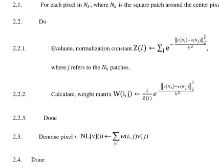
2.1. For each pixel in 𝑁_𝑘, where 𝑁_𝑘 is the square patch around the center pixel k,

2.2. Do

2.2.1. Evaluate, normalization constant

Z(𝑖) ← e

−

𝑣 _𝑁𝑖_{−𝑣(𝑁𝑗)}₂2

ℎ2

j

,

where j refers to the 𝑁𝑘patches.

2.2.2. Calculate, weight matrix

W i, j ←

1 𝑍(𝑖)

𝑒

− 𝑣 𝑁𝑖 −𝑣(𝑁𝑗 ) 2

2

ℎ2

2.2.3. Done

2.3. Denoise pixel i:



  I j ) ( ) , (

NL[v](i) w i j v j

2.4. Done

Figure 2-2 shows an example of the patch similarity measure for the NLM algorithm.

Here, the reference patch p is compared with its neighboring patches q1, q2 and q3. As

q1 and q2 are more similar to the reference patch p than q3, their weights, i.e. w(p, q1) ,

(24)

8

Figure 2-2: The Non-Local Means scheme where similar patches q1 and q2 are

assigned weights larger than q3.

In the NLM algorithm, when a patch size is M × M , the search region size is p × p, and

the image size is K × K, the complexity of the NLM algorithm will be 𝑂(𝑝2𝑀2𝐾2).

2.4 Applications of Non-Local Means

The Non-Local Means algorithm has been used in many applications. It has been used in

medical imaging such as on MR brain image [14][15], CT scan image [16], 3D

ultrasound imaging [17][18], diagnosis of heart echo images [19] . It has been used in

other applications such as video denoising [20][21][22], SAR image denoising [23][24],

(25)

9

2.5 Improvement over Non-Local Means

Many improvements have been suggested on the Non-Local Means algorithm in recent

years. Most of the significant improvements on the Non-Local Means algorithm have

been done using the patch regression, probabilistic early termination, a patch based

dictionary, neighborhood classification, principal component analysis and cluster trees. In

this section, we have described them briefly.

Bhujle [9] proposed a dictionary based denoising in which patches with similar

photometric structures are clustered together to create groups. Here, they build a

dictionary prior to denoising which can be accessed at a constant time. In their proposed

method, they build a global dictionary from all test images. Their approach can find

almost similar patches from the global dictionary in a short amount of time instead of

searching around the whole search window.

To search inside the dictionary, they build a tree data structure where searching starts

from the root node and calculate the distance between the reference patch. They also

suggested another improvement related to the patch edges. It improves the space and time

complexity by storing the residual image into the dictionary.

The proposed dictionary based NLM and their improvements on edge patch based

dictionary outperforms the original NLM by preselecting the similar patches and

performs denoising based on the calculated weights. In addition, edge patch based

dictionary reduces space and time to perform denoising by preselecting similar patches

based on residual edge image.

Mahmoudi et al. [10] accelerate the NLM algorithm by pre-classifying neighborhood

patches based on average gray values, gradient orientation, or both.

Chaudhury et al. [6] claimed that the denoising performance of the Non-Local Means

(26)

10

Vignesh et al. [7] proposed a speed up technique for the Non-Local Means algorithm

based on a probabilistic early termination (PET). In the original Non-Local Means

algorithm [4] distance calculation takes a significant amount of time. Neighborhood

selection can be done earlier using a soft decision. Contributing pixels can be rejected

when the expected distance value is below the weighted average. Probability models

based on patch features are used at each stage of distance computation to accept or reject

a patch. This scheme is called the probabilistic early termination (PET) scheme.

Tasdizen et al. [12] proposed principal component based Non-Local Means algorithm

where a global feature space is created to select important features. Image patches are

projected into the lower dimensional feature space and the dimensionality is reduced.

This reduced feature space is used for similarity measure rather than the entire feature

space.

Here, they proposed PCA to reduce the dimensionality of this feature space. PCA is

applied on the global feature space rather than on local feature space to provide an

efficient algorithm. They sort the eigenvectors in a descending order of eigen values and

projected the image patches into the lower subspace.

Reduced feature space gives better results over the original NLM denoising algorithm

and the author claims that it performs better in all cases. PCA is a data driven approach

and can adapt to a given image.

Brox et al. [13] proposed a technique to improve the performance of the NLM method

using a clustering tree. Here they introduced two novel techniques for NLM. Firstly, they

have introduced clustering tree for the Non-Local Means algorithm which allows a fast

pre-selection. It performs faster when the NLM algorithm considers the whole image as a

search region and works better for a fixed window size. Secondly, they have introduced

(27)

11

2.6 T-test

A hypothesis is a statement or claim about the state of an incident e.g. state of nature,

scientific investigation, market analysis, weather prediction which is unknown. Statistical

hypothesis is stated in terms of population parameters e.g. population mean and variance.

Researchers gather data and look for evidence to support or contradict about it. Testing a

hypothesis refers to accumulating relevant information and making a decision about the

action to be taken about the hypothesis. Testing a statistical hypothesis involves (1)

determination of test statistics and (2) utilization of the sample values of the statistics.

The test is performed to chose either a given hypothesis (called null hypothesis H0 ) or a

competing hypothesis (called alternate hypothesis 𝐻₁).

Let, testing procedure comprises that a statistics is a function of several random variables

𝑋₁, 𝑋₂, … , 𝑋_𝑛which gives,

𝑉 = 𝑉(𝑋₁, 𝑋₂, … , 𝑋_𝑛) (2.6)

Based on the observed random samples V, it decides to choose hypothesis between Ho or

H1. In respect to the distribution of V, two regions are chosen. Accepted region consists

of the values who adopt null hypothesis Ho. Rejected regions adopt alternate

hypothesis 𝐻₁. Here the main terminology is to decide whether a null hypothesis Ho is

accepted or rejected.

The population random variable X is a part of the competing hypotheses and their

distribution is not fully known. The observation of V leads to a decision regarding the

chosen hypothesis. For example, if a random variable contains a parameter θ, which may

have two observation 𝜃₀or 𝜃₁, The test statistics helps to decide whether to accept or

reject θ. For 𝜃₀as null hypothesis, we can write the following equations to represent

hypothesis testing problem.

𝐻_𝑜: 𝜃 = 𝜃₀ (2.7)

(28)

12

Possible outcome of the test is divided into two classes. One in the acceptance region A

and other in the critical region or rejection region B. Finally, if V falls in region A then

𝐻_𝑜is accepted and if it falls in B then 𝐻_𝑜is rejected.

It can be well explained using an example. Suppose that there are two identical boxes of

jelly beans. Box 1 contains 60 red jelly beans and 40 green jelly beans. Box 2 contains 40

red jelly beans and 60 green jelly beans. The proportion of red jelly beans p, for these two

boxes are

Box 1: p= 0.60

Box 2: p= 0.40

Suppose that there is a box on a table, but we do not know which one it is. We assume

that it is box 2, but we are not sure about that. To test our hypothesis that the box 2 is on

the table or not, we pick 10 random jelly beans. The number of red jelly beans in the test

samples will be used to decide whether box 2 is on the table or not.

W.S. Gosset derived the probability distribution for this statistics which named as

“student’s t” or simply t distribution. Figure 2-3 shows the student t distribution. This

function has only one parameter named degree of freedom. That is why t distribution

with v degree of freedom is called t(v) which is quite similar to the normal distribution

having bell shaped curve. The difference between normal distribution and t distribution is

that t distribution has a fatter tail over the normal distribution. This concluded as t

distribution has more probability in the extreme tail over the normal distribution. This

characteristic persists as for small value of the degree of freedom but it reduces as degree

of freedom exceeds 30 or more. When the degree of freedom is infinite, t distribution is

(29)

13

Figure 2-3: Student t distribution

In summary, we have discussed Gaussian noise, image denoising domains, the Non-Local

Means algorithm, as well as its variants. In addition we have discussed statistical t-test in

(30)

Chapter 3:Methodology

14

Chapter 3 Methodology

Non-Local Means is one of the most popular and powerful image denoising algorithm

available in recent years. It performs denoising in spatial domain and improves visual

quality of a noisy image. It can preserve edges and fine details. It denoises the center

pixel inside a reference patch by calculating a weighted average. Patches similar to the

reference patch contribute into this averaging process. In our thesis, we have reduced the

computational time to find similar patches by reducing the feature space.

3.1 Improved Non-Local Means Algorithm

Non-Local Means algorithm needs to search its neighboring area to find similar patches.

The utilized image patch size is usually 5×5, 7×7 or 9×9, which can be represented by 25,

49 or 81 dimensional feature vectors, respectively. This feature vector space is used to

assess the similarity between patches. In our proposed algorithm, a global feature vector

space is created in a preprocessing step (step 1). After that, a statistical test called t-test is

performed on this global feature vector space to reduce its dimensionality (step 2). This

reduced feature vector space is used during the rest of the denoising process.

3.1.1 Preprocessing

In the first step, we have created a feature vector space for the noisy image. An image

patch is linearized and represented as a row vector of size j. Thus the dimension of this

feature vector space will be j× N, where N is the total number of pixels in an image.

(31)

15

(3.1)

Here, for example if we have a patch size of 7×7 then j will be equal to 49. This matrix

will be used during the dimensionality reduction process.

3.1.2 T-test

We have implemented a paired t-test of the null hypothesis. This test is performed on the

matrix C. For each test case (i.e., each column in the matrix C), once the t value is

determined, the students t-distribution lookup table is used to find the value of p. When

the calculated p value is below a given threshold value, then the null hypothesis is

rejected. In our denoising problem, we have considered each patch as a feature vector.

The hypothesis tries to accept or reject a feature (i.e. an entire column in the matrix C).

Here, the null hypothesis is whether a feature is significant or not. In calculating the null

hypothesis, one uses the following normalization equation

𝑇 =

𝑥 −µ0

𝑠 𝑛 (3.2)

Where, 𝑥 is the sample mean,

µ

₀ is the population mean, s is the sample standard

deviation and n is the sample size. When the null hypothesis is accepted, it concludes that

the feature is significant. Otherwise, this feature is not significant. Thus the entire column

is deleted and hence reduces the size of matrix C.

(32)

16

3.1.3 Non-Local Means algorithm

In the Non-Local Means algorithm, a discrete noisy image v= {v (i) |i ϵ I}, where I is the

input image, can be denoised by calculating the weighted average,

𝑁𝐿 𝑣 𝑖 = 𝑤 𝑖, 𝑗 𝑣(𝑗)𝑗𝜖𝐼 (3.3)

Here, the weight w (i , j) depends on the similarity between the pixel i and the pixel j of

the intensity gray level vectors 𝑣(𝑁_𝑖) and 𝑣(𝑁_𝑗). Here, 𝑁_𝑘 is the square patch around the

center pixel. This weight is assigned to value v(j) which denoises pixel i. It can be

computed as,

𝑤 𝑖, 𝑗 =

1 𝑍(𝑖)

𝑒

− 𝑣 𝑁𝑖 −𝑣(𝑁𝑗 ) 2

2

ℎ2 _(3.4)

Here, h is the smoothing kernel width which controls the decay of the exponential

function.

𝑣

𝑁

_𝑖

− 𝑣(𝑁

_𝑗

)

2 2

is the Euclidean distance between two pixels i and j. Z(i) is

a normalization constant calculated as,

Z(𝑖) = e

−

𝑣 𝑁𝑖 −𝑣(𝑁𝑗 ) 22 ℎ2

j (3.5)

We have reduced the size of the feature vector over the original NLM algorithm. In our

proposed method 𝑁_𝑘 is replaced by 𝑓_𝑘, where 𝑓_𝑘 is the reduced feature vector. Then we

(33)

17

Our proposed algorithm is summarized as follows.

Algorithm Improved Non-Local Means

Input I:Image with additive white Gaussian noise

Output NL(I): Denoised image

1. Crate a global feature matrix C (as shown in Equation 3.1).

2. Perform the t-test on matrix C to produce the reduced row matrix 𝑓_𝑘.

3. For each pixel i, where i ϵ [1, N],

4. Do

4.1. For each pixel in 𝑁_𝑘, where 𝑁_𝑘 is the square patches around the center pixel k,

4.2. Do

4.2.1. Evaluate the normalization constant Z(𝑖) ← e− 𝑣 𝑓𝑖 −𝑣(𝑓𝑗 ) 2 2 ℎ 2

j ,

where j refers to the 𝑁_𝑘 patches.

4.2.2. Calculate the weight matrix

W i, j ←

1 𝑍(𝑖)

𝑒

− 𝑣 𝑓𝑖 −𝑣(𝑓𝑗 ) 2 2

ℎ2

4.2.3. Done

4.3. Denoise pixel i:



  I j ) ( ) , (

NL[v](i) w i j v j

(34)

18

3.1.4 Parameter Setting

Our proposed algorithm depends on the following parameters,

1. Patch size,

2. Search region size,

3. Threshold value.

We have analyzed the effect of these parameters on our test images and reported their

comparative performance in terms of PSNR (see Section 4.3.1) in the following sections.

Figure 3-1 shows the test images used in our experiment.

(a) Bridge (b) Columbia (c) Lake (d) Lax

(e) Milk drop (f) Plane (g) Woman 1 (h) Woman 2

(35)

19

3.1.4.1 Patch Size

Large patch size suppresses small details whereas small patch size fails to denoise

properly. Yet in the case of large patch size, it is difficult to find patches similar to the

reference patch, as such repeated patterns may appear less frequently.

In our experiment we have three parameters. Here, we have fixed the size of search

region and the threshold value. We have taken the search region of size 21×21 and the

threshold value 5. Then we have analyzed the effect of different patch sizes on our test

images at various noise levels.

Table 3-1 shows the effect of various patch sizes on our test images and reported their

average PSNR values over all test images at various noise levels. It has been found that,

patch size 7×7 works better for noise level σ<80 and patch size 5×5 works better for

higher noise levels.

Figure 3-2(a) - (d) show the effect of patch sizes 5×5, 7×7, 9×9 and 11×11, respectively

on Woman 1 image for noise level σ=40 . It has been found that Figure 3-2 (b) performs

(36)

20

Table 3- 1: Average PSNR comparison for all test images between different patch sizes

for different noise levels.

Noise Level 3×3 5×5 7×7 9×9 11×11

Search region sizes 21×21, threshold value = 5

10 32.10 33.62 33.75 32.93 32.08

20 29.25 30.42 30.60 29.88 29.07

30 27.51 28.67 28.78 28.09 27.27

40 26.29 27.33 27.49 26.83 25.91

50 25.42 26.42 26.54 25.94 25.04

60 23.18 24.11 24.27 23.67 23.10

70 21.93 22.99 23.03 22.45 22.08

80 21.49 22.52 22.25 21.94 21.52

90 20.78 21.76 21.74 21.09 20.85

(37)

21

(a) (b)

(c) (d)

Figure 3 - 2: Performance analysis using Woman 1 image over different patch sizes

where noise level is σ=40. (a) patch size 5×5, PSNR = 29.55, (b) patch size 7×7, PSNR =

(38)

22

3.1.4.2 Search Region Size

Large search region size helps to find more patches similar to the reference patch.

Whereas, small search region size faces difficulty to find enough similar patches.

Here, we have fixed the size of the threshold value. We have taken the patch sizes from

Section 3.1.4.1. For noise level σ<80, we have chosen patch size 7×7 and the threshold

value 5. For noise level σ>80, we have chosen patch size 5×5 and the threshold value 5.

Then we have observed the effect of different search region sizes over all test images at

various noise levels.

Table 3-2 shows the effect of search region sizes on our test images and reported their

average PSNR values. It has been found that, for patch size 7×7 and noise level σ<80, the

search region sizes 21×21, 28×28 and 35×35 perform the best. For patch size 5×5 and

noise level σ>80, the search region sizes 15×15, 20×20 and 25×25 show the best

performance. We have selected the minimum search region size for each case to reduce

complexity.

Figure 3-3 (a)-(d) show the effect of search region sizes 14×14, 21×21, 28×28 and 35×35,

respectively on Woman 1 image for noise level σ=40. Figure 3-3 (b), (c) and (d) show

(39)

23

Table 3- 2: Average PSNR comparison for all test images between different search

region sizes for different noise levels.

Noise Level 14×14 21×21 28×28 35×35

Patch size 7×7, threshold value = 5

10 32.12 33.75 33.75 33.75

20 29.34 30.60 30.60 30.61

30 27.60 28.78 28.78 28.78

40 26.37 27.49 27.49 27.49

50 25.47 26.54 26.54 26.55

60 23.26 24.27 24.27 24.27

70 22.08 23.03 23.03 23.04

Noise Level 10×10 15×15 20×20 25×25

Patch size 5×5, threshold value = 5

80 21.45 22.52 22.52 22.52

90 20.86 21.75 21.75 21.76

(40)

24

(a) (b)

(c) (d)

Figure 3 - 3: Performance analysis using Woman 1 image over different search region

sizes where noise level is σ=40 (a) search region size=14×14, PSNR = 29.11, (b) search

region size=21×21, PSNR = 29.78, (c) search region size=28×28, PSNR = 29.78, and (d)

(41)

25

3.1.4.3 Threshold value

The threshold value determines whether a hypothesis is accepted or rejected. Here, we

have analyzed the effect of this threshold value for different noise levels.

Here, we have chosen parameters form the Section 3.1.4.1 and Section 3.1.4.2. For a

noise level σ<80, we have chosen the patch size 7×7 and the search region size 21×21. For noise level σ>80, we have chosen the patch size 5×5 and the search region size

15×15. Then we have observed the effect of different threshold values over all test

images at various noise levels.

Table 3-3 and Table 3-4 show the value of average PSNR and the average number of

features selected for each noise levels at various threshold values. Here, the threshold

value represents the percentage of rejection. The bolded PSNR values represent the best

results among these two tables. If we check the values from these two tables, we can find

that the threshold value 3 and the threshold value 5 show the best result for the noise

levels σ<80, patch size of 7×7 and for the noise levels σ>80, patch size of 5×5,

respectively. We have chosen threshold value 5 as it requires fewer features to produce

the same result.

Figure 3-4 and Figure 3-5 show the average PSNR and the average number of features

for the patch size 7×7 for the threshold value 3 and the threshold value 5, respectively

over all test images at various noise levels. Figure 3-6 and Figure 3-7 show the average

PSNR and the average number of features for the patch size 5×5 for threshold value 3 and

the threshold value 5, respectively. Figure 3-8 (a)-(d) show the effect of the threshold

values at 3,5,7 and 9, respectively on Woman 1 image for noise level σ=40. It has been

(42)

26

Table 3- 3: Average PSNR and average number of features comparison for patch size

7×7 for all test images between different threshold values for different noise levels.

Noise Level

3 5 7 9 11

Patch size 7×7, search region size 21×21

10 PSNR 33.75 33.75 33.51 33.31 33.12

# of Features

Size

42.13 39.38 36.88 35.38 33.63

20 PSNR 30.60 30.60 30.39 30.21 30.02

# of Features

Size

40.38 38.13 35.75 33.88 32.75

30 PSNR 28.79 28.78 28.54 28.41 28.12

# of Features

Size

39.75 37.13 35.75 33.63 31.75

40 PSNR 27.48 27.48 27.30 27.24 27.10

# of Features

Size

39.13 36.88 34.63 32.76 30.75

50 PSNR 26.54 26.54 26.33 26.25 26.10

# of Features

Size

38.5 36 33.89 32.63 30.63

60 PSNR 24.27 24.27 24.11 23.95 23.85

# of Features

Size

37.75 35.38 33 32.5 30.38

70 PSNR 23.03 23.03 22.94 22.85 22.69

# of Features

Size

37.63 35.73 32.88 31.75 29.5

80 PSNR 22.26 22.26 22.24 22.18 22.11

# of Features

Size

36.88 33.87 31 29.88 28.5

90 PSNR 21.74 21.74 21.71 21.66 21.58

# of Features

Size

36.5 33.88 30.88 29.75 28.38

100 PSNR 21.07 21.06 21.08 20.98 20.96

# of Features

Size

(43)

27

Table 3- 4: Average PSNR and average number of features comparison for patch size

5×5 for all test images between different threshold values for different noise levels.

Noise Level

3 5 7 9 11

Patch size 5×5, search region size 15×15

10 PSNR 33.61 33.61 33.57 33.56 33.55

# of Features

Size

24.17 23.5 23.17 22.83 22.17

20 PSNR 30.38 30.37 30.36 30.33 30.31

# of Features

Size

24.17 23.5 22.83 22.67 21.83

30 PSNR 28.65 28.64 28.61 28.60 28.59

# of Features

Size

23.83 23 22.67 22.5 21.83

40 PSNR 27.32 27.31 27.31 27.30 27.29

# of Features

Size

23.83 22.83 21.83 21.67 20.83

50 PSNR 26.41 26.41 26.40 26.39 26.38

# of Features

Size

23 22.67 21.83 21 20.83

60 PSNR 24.10 24.10 24.09 24.08 24.07

# of Features

Size

23 21.83 21 20 19.67

70 PSNR 22.98 22.97 22.97 22.96 22.95

# of Features

Size

22.67 21.83 20.83 19.17 18.83

80 PSNR 22.52 22.52 22.33 22.15 21.94

# of Features

Size

22.67 21 19 19 17.83

90 PSNR 21.76 21.76 21.50 21.34 21.11

# of Features

Size

21.83 20.83 19 18 17.33

100 PSNR 21.12 21.12 20.91 20.81 20.73

# of Features

Size

(44)

28

Figure 3 - 4: Average PSNR and average number of features comparison for patch size

7×7 and threshold value 3 over different noise levels.

7×7 and threshold value 5 over different noise levels. 0 5 10 15 20 25 30 35 40 45

10 20 30 40 50 60 70 80 90 100

A ve rag e Value s Noise Levels PSNR

Number of Features

0 5 10 15 20 25 30 35 40 45

10 20 30 40 50 60 70 80 90 100

(45)

29

5×5 and threshold value 3 over different noise levels.

5×5 and threshold value 5 over different noise levels. 0 5 10 15 20 25 30 35 40

10 20 30 40 50 60 70 80 90 100

Number of Features

0 5 10 15 20 25 30 35 40

10 20 30 40 50 60 70 80 90 100

(46)

30

(a) (b)

(c) (d)

Figure 3 - 8: Performance analysis using Woman 1 image over differentthreshold values

where noise level is σ=40 and patch size is 7×7 (a) threshold value 3, PSNR = 29.79, (b)

threshold value 5, PSNR = 29.79, (c) threshold value 7, PSNR = 29.33, and (d) threshold

(47)

31

3.1.5 Selected Parameters

To confirm the performance of our selected parameters, we have evaluated the effect of

patch size by keeping the value of search region size and the threshold value constant.

Table 3-5 shows the effect of patch sizes while the search region size is 21×21 and the

threshold value is 5. It has been found that the patch size 7×7 performs the best. Table

3-6 shows the effect of patch size while the search region size is 15×15 and the threshold

value is 5. It has been found that patch size 5×5 performs the best. The bolded PSNR

value represents the best results among these two tables. It has been found that for noise

level σ<80, patch size 7×7 performs the best and for noise level σ>80, patch size 5×5

performs the best among these two tables.

Noise level estimation can be performed before assigning these parameters.

Pre-classification of homogeneous areas [28] [29], image filtering [30] [31], Wavelet

transform [32] and local variance estimate [33] are most widely used models to estimate

the noise from an image.

Finally, we can conclude that for noise level σ<80, patch size 7×7 performs the best.

Whereas for noise level σ>80, patch size 5×5 performs the best (see Section 3.1.4.1). For

patch size 7×7, search region size 21×21 performs the best and for patch size 5×5, search

region size 15×15 performs the best (see Section 3.1.4.2). Threshold value 5 shows the

(48)

32

Noise Level 3×3 5×5 7×7

9×9

11×11

Search region size 21×21, threshold value = 5

10 32.09 33.62 33.75 32.91 32.06

20 29.21 30.43 30.60 29.88 29.07

30 27.52 28.64 28.78 28.07 27.28

40 26.27 27.31 27.49 26.81 25.90

50 25.41 26.41 26.54 25.92 25.03

60 23.18 24.11 24.27 23.67 23.10

70 21.93 22.99 23.03 22.45 22.08

80 21.49 22.13 22.48 21.97 21.52

90 20.78 21.38 21.65 21.13 20.85

(49)

33

Noise Level 3×3 5×5 7×7

9×9

11×11

Search region size 15×15, threshold value = 5

10 32.07 33.67 33.43 32.42 32.09

20 29.21 30.39 30.31 29.41 29.07

30 27.52 28.64 28.50 27.70 27.28

40 26.30 27.32 27.23 26.46 25.91

50 25.42 26.40 26.28 25.58 25.04

60 23.18 24.10 24.03 23.35 23.10

70 21.93 22.98 22.80 22.13 22.08

80 21.41 22.52 22.23 22.09 21.47

90 20.71 21.76 21.41 21.27 21.11

(50)

Chapter 4:Experimental Results and Analysis

34

Chapter 4 Experimental Results and Analysis

We have tested our image denoising algorithm on a standard image set with noise

standard deviation σ ranging from 10 to 100 for additive white gaussian noise. We have

compared our proposed method with the Non-Local Means algorithm as well as its

variants. We have compared our results and analyzed it based on the PSNR and the SSIM

measures. We also analyzed and compared the results subjectively.

4.1 Data set

We have used standard images for our test purpose. Figure 4-1 shows the test images.

These standard images are initially noise free. We contaminated them with additive white

gaussian noise for testing purpose.

4.2 Noise Generation

Noise can be defined as a deviation from the ideal signal. In general, additive noise is

evenly distributed over the original image. To generate a noisy image for our testing

purpose, the generated noise is added to the original image. The final signal is kept under

the maximum range of intensity value of gray image. Figure 4-2 shows the example of a

(51)

35

(a) Lena (b) Man (c) Boat (d) Baboon

(e) Barbara (f) Peppers (g) Hill (h) Couple

Figure 4- 1: Set of images for performance analysis.

4.3 Performance measure

To evaluate the performance of our denoising algorithm we have used the Peak Signal to

Noise Ratio (PSNR) and the Structural Similarity (SSIM) measure. These are widely

(52)

36

(a) (b)

Figure 4- 2: Noise generation (a) Noise free image Lena. (b) Noisy image with Additive

white Gaussian noise (noise level σ=50).

4.3.1 Peak Signal to Noise Ratio

The peak signal to noise ratio (PSNR) represents the ratio between the maximum powers

of a signal to the noise which degrades the original image. This measure is based on the

Mean Squared Error (MSE) which assesses the difference between the original image

data and the degraded image data. Given the original image data 𝑢_𝑖𝑗 and the degraded

image data 𝑣_𝑖𝑗 of size M×N, MSE is defined as,

𝑀𝑆𝐸 =

1

𝑀×N

(𝑢

𝑖𝑗

− 𝑣

𝑖𝑗

)

2 𝑁

𝑗 =0 𝑀

𝑖=0 (4.1)

𝑃𝑆𝑁𝑅 = 10 log

₁₀ 𝑀𝐴𝑋

2

(53)

37

where MAX is the maximum possible pixel intensity value. High PSNR value indicates a

better reconstruction or denoising. The drawback of PSNR is that it relies only on pixel

numerical values rather than any structural similarity.

4.3.2 Structural Similarity Index (SSIM)

The structural similarity index is used to find similarity between two images. Similar

pixels have strong inter-dependencies when they are closer. The following equation

measures SSIM

𝑆𝑆𝐼𝑀 =

(2µ𝑥µ𝑦+𝑐1)(2𝜎𝑥𝑦+𝑐2)

(µ_𝑥2+µ_𝑦2+𝑐₁)(𝜎_𝑥2+𝜎_𝑦2+𝑐₂) (4.3)

Where, x and y are two windows of identical size. In this equation

µ

_𝑥 and

µ

_𝑦 are the

average of x and y, 𝜎𝑥2 and 𝜎𝑦2 are the variance of x and y and 𝜎𝑥𝑦 is the co-variance.

𝑐1 = (𝑘1𝐿)2 and 𝑐2 = (𝑘2𝐿)2; 𝑘1 ≪ 1 , 𝑘2 ≪ 1 and L is the dynamic range of pixel

values.

4.4 Results and Analysis

4.4.1 Parameter Setting

The performance of the proposed method is assessed using peak signal to noise ratio

(PSNR) and the structural similarity measure (SSIM). For noise levels σ<80, we have

considered the patch size to be 7×7, the search region size to be 21×21 and the threshold

value to be 5. For noise levels σ>80, the patch size is set to be 5×5, the search region size

is set to be 15×15 and the threshold value is set to be 5 (see Section 3.1.5). During the

rest of our results and analysis we have used these parameters for our proposed method.

We have used Matlab R2013b (version 8.2.0.29) for our implementation purposes. All of

(54)

38

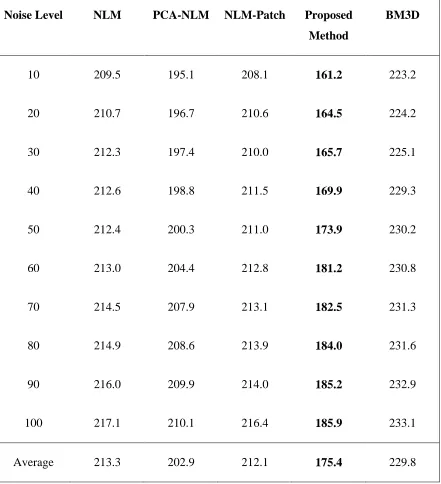
under Linux OS using Ubuntu 14.1. The execution time was recorded in milliseconds. All

of the test results are recorded and averaged after 10 runs.

4.4.2 Performance analysis using PSNR

The performance of our proposed method is compared in terms of PSNR with other

denoising schemes, namely the original NLM method, the principal component analysis

based NLM method (PCA-NLM), the patch regression based NLM method (NLM-

Patch) and the BM3D method.

Table 4-1 and Table 4-2 show the comparative performance for Lena image and the

average comparative performance for all test images at different noise levels,

respectively. The bolded values represent the highest PSNR value among all of the

algorithms for a given noise level. Figure 4-3 compares the average PSNR for the

proposed method and all other denoising algorithms.

It has been found that, the proposed method performs better than all other methods except

BM3D. In case of the BM3D method, the proposed method performs better than the

BM3D method only when σ<50. The BM3D method performs better at the higher noise

(55)

39

Table 4-1: PSNR(dB) comparison for Lena image among the proposed method, the

NLM method, variants of the NLM method and the BM3D method for different noise

levels.

Noise Level NLM PCA-NLM NLM-Patch Proposed

Method

BM3D

10 34.57 34.58 33.21 35.91 35.79

20 31.89 31.92 30.09 33.32 32.94

30 30.0 31.05 27.71 31.55 31.16

40 28.42 29.02 25.85 29.97 29.79

50 27.10 26.99 25.46 27.65 28.70

60 25.55 24.98 23.89 25.98 28.27

70 23.99 24.01 23.10 24.93 27.57

80 23.05 23.51 22.82 23.96 26.97

90 22.99 22.98 21.95 23.09 26.45

100 22.18 22.19 21.17 22.29 25.95

(56)

40

Table 4-2: Average PSNR(dB) comparison for all test images among the proposed

method, the NLM method, variants of the NLM method and the BM3D method for

different noise levels.

Noise Level NLM PCA-NLM NLM-Patch Proposed

Method

BM3D

10 32.52 32.94 31.47 33.94 33.84

20 29.87 29.95 29.04 31.0 30.50

30 28.13 28.26 27.45 28.96 28.38

40 26.69 26.43 25.87 27.72 27.70

50 25.49 25.38 24.61 26.49 26.86

60 23.85 23.87 22.75 24.30 25.94

70 22.90 22.81 22.31 23.22 25.29

80 22.32 22.32 21.92 22.60 24.75

90 21.73 21.57 20.89 21.86 24.18

100 21.13 20.94 20.14 21.19 23.68

(57)

41

Figure 4- 3: Bar graph for average PSNR comparison for the proposed method, the NLM

method, variants of the NLM method and the BM3D method for different noise levels.

4.4.3 Performance analysis using SSIM

Table 4-3 and Table 4-4 show the SSIM comparison for Lena image and the average

SSIM comparison for all test images between the proposed method and the other

denoising schemes, respectively. The bold face digits represent the highest SSIM value

among all of these algorithms. Figure 4-4 compares average SSIM between the proposed

method and other the denoising schemes.

For noise level σ<50, the proposed method performs better than all other denoising

schemes. Yet, for noise level σ>50 the proposed method performs better than the original

NLM and its variants. The BM3D performs better at higher noise levels.

Appendix A exhibits further analysis on Pepper, Boat and Couple image. 18 19 20 21 22 23 24 25 26 27 28 29 30 31 32 33 34 35

10 20 30 40 50 60 70 80 90 100

PS N R v al u e

Noise Standard Deviation, σ

NLM

PCA NLM

NLM-Patch

Proposed Method

Improved Non-Local Means Algorithm Based on Dimensionality Reduction