The Near Wake of a European Starling

(1)

Western University Western University

Scholarship@Western

Electronic Thesis and Dissertation Repository

12-11-2012 12:00 AM

The Near Wake of a European Starling

Adam J. Kirchhefer

The University of Western Ontario

Supervisor Dr. Greg Kopp

The University of Western Ontario

Graduate Program in Mechanical and Materials Engineering

A thesis submitted in partial fulfillment of the requirements for the degree in Doctor of Philosophy

Follow this and additional works at: https://ir.lib.uwo.ca/etd

Part of the Aerodynamics and Fluid Mechanics Commons, and the Biology Commons

Recommended Citation Recommended Citation

Kirchhefer, Adam J., "The Near Wake of a European Starling" (2012). Electronic Thesis and Dissertation Repository. 1016.

https://ir.lib.uwo.ca/etd/1016

This Dissertation/Thesis is brought to you for free and open access by Scholarship@Western. It has been accepted for inclusion in Electronic Thesis and Dissertation Repository by an authorized administrator of

(2)

THE NEAR WAKE OF A EUROPEAN STARLING

(Thesis format: Monograph)

by

Adam Jonathon Kirchhefer

Graduate Program in Mechanical and Materials Engineering

A thesis submitted in partial fulfillment of the requirements for the degree of

Doctor of Philosophy

The School of Graduate and Postdoctoral Studies The University of Western Ontario

London, Ontario, Canada

(3)

ii

THE UNIVERSITY OF WESTERN ONTARIO School of Graduate and Postdoctoral Studies

CERTIFICATE OF EXAMINATION

Supervisor

______________________________ Dr. Gregory Kopp

Supervisory Committee

______________________________ Dr. Eric Savory

Examiners

______________________________ Dr. Craig Miller

______________________________ Dr. Kamran Siddiqui

______________________________ Dr. Anthony Straatman

______________________________ Dr. Pierre Sullivan

The thesis by

Adam Jonathon Kirchhefer

entitled:

The Near Wake of a European Starling

is accepted in partial fulfillment of the requirements for the degree of

Doctor of Philosophy

______________________ _______________________________

(4)

iii

Abstract

The wake of a freely flying European starling (Sturnus vulgaris) was measured using high

speed, time-resolved, particle image velocimetry, simultaneously with high speed

cameras which imaged the bird. These measurements have been used to generate vector

maps in the near wake that can be associated with the bird’s location and wing

configuration. A kinematic analysis has been performed on select sequences of

measurements to characterize the motion of the bird, as well as provide a point of

comparison between the bird of the present study and other birds or flapping wings. Time

series of measurements have been expressed as composite wake plots which relate to

segments of the wing beat cycle for various spanwise locations in the wake. The wake

composites invoke Taylor’s Frozen Flow Hypothesis. The applicability of Taylor’s

Frozen Flow Hypothesis to the starling wake is discussed and evaluated. Measurements

of the wake indicate that downwash is not produced during the upstroke, suggesting that

the upstroke does not generate lift. Additional characteristics of the wake are discussed

which imply the presence of (secondary) streamwise vortical structures, in addition to the

wing tip vortices. The lack of downwash during the upstroke and the suggestion of

secondary streamwise vortical structures constitute a deviation from a wake model which

has been developed and supported by other bird species. Furthermore, these flow features

indicate similarities between the wakes of birds and bats. In light of recent studies

reported in the literature, the presence of secondary streamwise vortical structures may

not only be a feature shared by birds and bats, but a general feature of flapping wings.

Measurements also show spanwise vortical structures a short distance downstream of the

(5)

iv

the bird, it is speculated that the wings of a starling may undergo dynamic stall during

flight. This is also implied by the results of the kinematic analysis of the bird’s wing

motion and comparison to other flapping wing studies. Dynamic stall, thought to be

limited to hovering and slow flight, would enable high efficiency and high force

coefficient generation.

Keywords

Bird flight, European starling, flapping wing, particle image velocimetry (PIV), near

(6)

v

Acknowledgements

I would like to thank Dr. Greg Kopp and Dr. Roi Gurka for their guidance, advice, and

support throughout this project. I am particularly grateful that they not only prompted me

to have the most influence I could have had on the work, but also, allowed the work to

have a significant influence on myself.

The completion of this work is the result of the kind contribution of many individuals. I

would like to thank Wayne Bezner Kerr for his invaluable help in the experiments, as

well as for sharing insight from his expertise in both the fields of biology and aviation.

The contributions of Eugene Porter and Dave Lunn to the electronic components of the

experiment were essential as well, and I am grateful they shared their interest as well as

their time.

Beyond numerous contributions to the work itself, I am grateful to many people for their

support. For this, to my parents Louise and Siegfried Kirchhefer, my sister Sara Sinclair,

(7)

vi

List of Tables

Table 1 – Morphological and experimental parameters ... 33

Table 2 – Morphology and kinematics of birds for which PIV wake data is available .... 57

Table 3 – Morphology and kinematics of the European starling and bats for which PIV

data is available ... 58

(11)

x

List of Figures

Figure 1.1 – A comparison of smoke flow visualizations. The free stream passes from left

to right. The flow field around a static wing is seen from the side in (a) from Babinsky

2003, with permission. The flow field of flapping wing at the end of its downstroke is

shown from the side in (b), reprinted by permission from Macmillan Publishers Ltd:

Nature, Taylor et al. (2003). ... 2

Figure 1.2 – Flow visualization and schematic representation of the wake of a chaffinch.

In (a), a chaffinch flies slowly through a cloud of wood and paper dust. In (b), the motion

of the dust has been interpreted as a vortex loop shed during the downstroke. Reprinted

by permission from Macmillan Publishers Ltd: Nature, Kokshaysky (1979). ... 4

Figure 1.3 – From Hedenström and Spedding (2008) Figure 1 page 596, original work by

Spedding et al. (2003). A schematic representation of the wake of a thrush nightingale

flying in the middle of its natural range of flight speeds. Tubes indicate vortical

structures generated by a bird as it flies from right to left. The blue and red tubes indicate

structures shed from the downstroke and the upstroke, respectively. ... 5

Figure 1.4 – From Hedenström et al. (2007) reprinted with permission from AAAS, a

schematic of the wake generated by a Pallas’ long-tongued bat as it flies through the air in

the direction indicated by the blue arrows. The blue and red tubes represent vortex

structures originating from the downstroke and upstroke, respectively. The structure is

representative of the wake at medium and fast speeds within the natural speed range of

the bat. ... 6

Figure 1.5 – From Hedenström and Spedding (2008) Figure 1 page 596, original work by

Henningsson et al. (2008). A schematic of the wake generated by a swift as it flies

through the air in the direction indicated by the blue arrow. Green tubes indicate wing tip

vortices. Red and blue tubes indicate the gradual shedding of vorticity throughout the

entire wing beat cycle. ... 7

Figure 1.6 - A summary of wake measurement locations from PIV studies of vertebrates

(12)

xi

measurement locations of (a)bird wakes and (b)bat wakes. Studies include the work of 1.

Spedding et al. (2003), 2. Hedenström et al. (2006), 3. Rosén et al. (2007), 4.

Henningsson et al. (2008), 5. Johansson and Hedenström (2009), 6. Henningsson et al.

2011, 7. Hedenström et al. 2007, 8. Johansson et al. 2008, 9. Hubel et al. (2009) and 10.

Hedenström et al. 2009.The streamwise (∆x) and spanwise (∆z) locations have been

normalized by the mean wing chord ,c , and semispan, bsemi, of the respective study. Solid

lines indicate that measurements were taken in a spanwise-normal plane. Dashed lines

indicate that measurements were taken in a streamwise-normal (Trefftz) plane. Dashed

rectangles indicate the range from which streamwise-normal measurements were taken.

Abbreviations used in the legend represent the lesser short-nosed fruit bat (LSNFB),

Pallas’ long-tongued bat (PLTB) and the southern long-nosed fruit bat (SLNB). ... 9

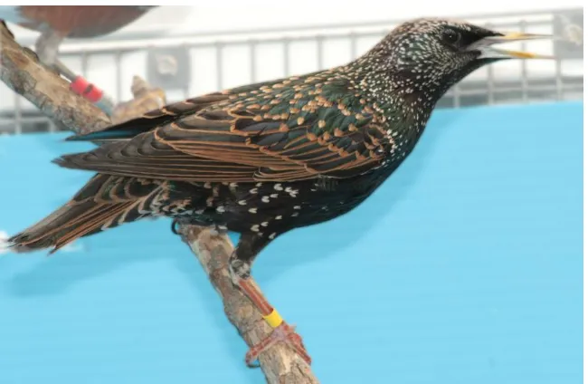
Figure 1.7 - A European starling used in the present study... 10

Figure 1.8 – A visual comparison of a (a) Pallas’ long-tongued bat (Fenton 2010) and a

(b) European starling ... 11

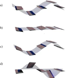
Figure 2.1 – A summary of flapping wing motion classes, including a) heaving, b)

pitching, c) combined heaving and pitching and d) rolling. A complete cycle of the

wing’s motion is shown as it travels from right to left. The trajectory of the wing is

indicated by the semitransparent blue surface. ... 13

Figure 3.1 – Schematic side view of the AFAR wind tunnel. ... 29

Figure 3.2 - Photograph of the empty test section of the AFAR wind tunnel. ... 29

Figure 3.3 - A scaled drawing of the experimental set-up in the wind tunnel. Part a) shows

the setup from the downstream end of the test section. Part b) shows a cross-section of

the setup, with the average flow passing from left to right. All dimensions are given in

millimeters. ... 30

Figure 3.4 - A comparison of the planform outline of the bird from Exp. 1 and Exp. 2. .. 34

Figure 3.5 – A photograph and schematic of custom made laser goggles used in Exp. 1,

(13)

xii

into a shape with 3 “lobes.” The two upper lobes fold over the bird’s head, and the lower

lobe is folded under the head. Once behind the head, the lobes are fastened together with

medical tape and elastic bands. ... 35

Figure 3.6 – A schematic representation of the KIN camera and SPAN camera fields of

view relative to the PIV field of view in the wind tunnel. Approximate dimensions are

given in millimeters. ... 36

Figure 3.7 - Simultaneous realization of the bird and the wake. Streak lines originating

from the wing root and wing tip have been added from a kinematic analysis after the

experiment. ... 39

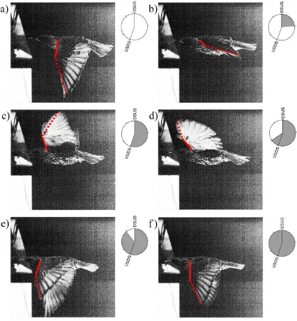
Figure 4.1 – A series of images depicting an entire wing beat cycle. The first (top left)

and last (bottom right) images show the wings at the end of the downstroke. The inset

beside each image shows the relative phase of each image with respect to the downstroke

to upstroke (DSUS) and the upstroke to downstroke (USDS) transition. The leading edge

of the arm wing is indicated by a solid red line. The leading edge of the hand wing is

indicated by a dashed red line. ... 44

Figure 4.2 – A view from upstream of the bird, light sheet, and camera viewing cone.

The path of the wing tip is indicated as a dashed line during the upstroke and a solid line

during the downstroke. Landmarks digitized for kinematic analysis are circled. During

the downstroke, the wing is treated as a rod of constant length, R, which rotates about the

shoulder joint. ... 46

Figure 4.3 – The position of the bird, represented by the position of the wing root, relative

to the PIV field of view for various measurement sequences. Measurement sequences in

the legend are described by the phase of the wing beat cycle and the spanwise offset of

the bird from the PIV measurement plane. ... 47

Figure 4.4 – The average velocity of the bird for various measurement sequences.

Measurement sequences are described by the phase of the wing beat cycle and the

(14)

xiii

Figure 4.5 – The angular position of the wing throughout the downstroke. The time at

which the wing finishes the downstroke and transitions to the upstroke is indicated as

tDSUS. The mean function of θ is indicated by a black line. ... 48

Figure 4.6 – The angular velocity of the throughout the downstroke. The time at which

the wing finishes the downstroke and transitions to the upstroke is indicated as tDSUS. The

mean function of Vθ is indicated by a black line. ... 49

Figure 4.7 – The longitudinal velocity of the wing tip relative to the air throughout the

downstroke. Values greater than 1 indicate the wingtip is traveling upstream. The time at

which the wing finishes the downstroke and transitions to the upstroke is indicated as

tDSUS. The mean function of Vx is indicated by a black line. ... 49

Figure 4.8 – An estimation of the wing’s maximum angle of attack from its instantaneous

pitch and velocity relative to the air. In a), the left wing of the bird points directly at the

camera, and the pitch of the chord line at approximately 2/3 bsemi is represented by the

blue line. In b), the pitch of the chord line and the velocity of the wing section at 2/3 bsemi

are used to estimate the angle of attack, α, as approximately 13o. ... 51

Figure 4.9 – From Anderson et al. (1998) with permission, a schematic representation of

the wake patterns observed in their experiment on heaving and pitching airfoils. In the

experiments, St = πk. The red rectangle indicates the region in which the present wing

operates. ... 53

Figure 5.1 – A schematic representation of a flow feature moving through the field of

view. The two measurements of the flow feature are compared with a spatial offset of X.

In a) Taylor’s hypothesis holds perfectly, and the spatially-averaged time correlation is 1. In b), Taylor’s hypothesis is not perfectly held and the value of C is consequently less

than 1. ... 64

Figure 5.2 – An evaluation of the spatially-averaged time correlation coefficient Cu for

several values of T. Each row shows a contour map of the spatially-averaged time

correlation, and the two instantaneous vector fields used for its calculation. The temporal

(15)

xiv

peak value of the spatially-averaged time correlation, in the X-Y plane, is indicated by a

black triangle. ... 66

Figure 5.3 - An evaluation of the spatially-averaged time correlation coefficient Cv for

several values of T. Each row shows a contour map of the spatially-averaged time

correlation, and the two instantaneous vector fields used for its calculation. The temporal

separation between vector fields (T) increases from the top row to the bottom row. The

peak value of the spatially-averaged time correlation, in the X-Y plane, is indicated by a

black triangle. ... 67

Figure 5.4 – The value of the spatially-averaged time correlation coefficient for a

sequence of measurements at a spanwise location of approximately 0.6 bsemi. In a), the

coefficient was calculated using the streamwise component of velocity. In b), the

coefficient was calculated using the vertical component of velocity. During this

sequence, a vortex shed from the downstroke to upstroke transition passes through the

field of view. ... 68

Figure 5.5 - The value of the spatially-averaged time correlation coefficient for a

sequence of measurements at a spanwise location of approximately 0.2 bsemi. In a), the

coefficient was calculated using the streamwise component of velocity. In b), the

coefficient was calculated using the vertical component of velocity. ... 69

Figure 5.6 - The value of the spatially-averaged time correlation coefficient for a

sequence of measurements at the centreplane of the wake. In a), the coefficient was

calculated using the streamwise component of velocity. In b), the coefficient was

calculated using the vertical component of velocity. ... 69

Figure 5.7 – A summary of the peak in the spatially-averaged time correlation for

temporal shifts, T, corresponding to a) 0.002 s, b) 0.004 s c) 0.006 s and d) 0.008 s. These

values of T are equivalent to roughly 2.5%, 5%, 7.5%, and 10% of the wing beat cycle

period. The number of occurrences of a peak, N, is indicated by the shade at a given

(16)

xv

velocity equivalent to the free stream velocity. Local peaks of relevance are indicated by

blue arrows. ... 71

Figure 5.8 - A summary of the peak in the spatially-averaged time correlation, based on

v’, for temporal shifts, T, corresponding to a) 0.002 s, b) 0.004 s c) 0.006 s and d) 0.008 s.

These values of T are equivalent to roughly 2.5%, 5%, 7.5%, and 10% of the wing beat

cycle period. The number of occurrences of a peak, N, is indicated by the shade at a

given location. A dashed line indicates the value of Xf/ U∞ corresponding to a convection

velocity equivalent to the free stream velocity. Local peaks of relevance are indicated by

blue arrows. ... 72

Figure 6.1 - An overview of the wake where the spanwise position at which the

measurements were taken is indicated by the green line plotted over the planform outline

of the bird. The wing tip and wing root traces are indicated by the dashed black lines. ... 76

Figure 6.2 - The wake created by the downstroke to upstroke transition, as indicated by

the wing tip trace (dashed black line). Measurements are taken at a spanwise location of

approximately 0.6bsemi. ... 77

Figure 6.3 - The wake generated by the downstroke to upstroke transition from Figure

6.2. Velocity vectors are superimposed above a contour map of swirling strength ... 78

Figure 6.4 - The wake generated by the downstroke to upstroke transition at a spanwise

position slightly inboard of the wing tips, at approximately 0.45bsemi. Contour levels are

the same as in Figure 6.2. ... 79

Figure 6.5 - The wake generated by the downstroke to upstroke transition from Figure

6.4. Velocity vectors are superimposed above a contour map of swirling strength, with

the levels the same as in Figure 6.3. ... 80

Figure 6.6 - The wake generated by the wing at spanwise locations near the body at

approximately 0.2bsemi. Vorticity at the downstroke to upstroke transition is still visible,

(17)

xvi

Figure 6.7 - The wake sampled at spanwise locations near the centre of the wake at

approximately 0.1bsemi. Characteristics of a “double branch structure” are observed. ... 81

Figure 6.8 - The wake generated by the downstroke to upstroke transition at

approximately the centreplane. In (a), DSUS vorticity is observed underneath the wake of

the body while in (b) the field of view is too high to show this feature. ... 83

Figure 6.9 - A wake composite of vectors superimposed over contours of swirling

strength. The “vortex” at the downstroke to upstroke transition is present, with its

swirling strength being similar in magnitude to the eddies above it. ... 83

Figure 6.10 - The wake generated by the upstroke to downstroke transition relatively

close to the wing tips, at approximately 0.5bsemi. ... 84

Figure 6.11 - The wake generated by the upstroke to downstroke transition at a spanwise

position of approximately 0.2bsemi. A double branch structure is observed. ... 85

Figure 6.12 - The wake generated by the upstroke to downstroke transition at the

approximate centreplane of the wake. ... 86

Figure 7.1 – A schematic of the wake generated by the bird during the DSUS transition of

the wing. Vortex tubes (red) were generated by the DSUS transition (semitransparent

bird) and are measured when the bird has started the upstroke (black bird). The tubes

consist of a tip vortex (TV), DSUS vorticity (DSUS V), streamwise vortical structures

near the body (SVS) and a relatively weak connection across the centreplane (C). ... 90

Figure 7.2 –A comparison of the peak spanwise vorticity measured in the wake of

flapping animals from several studies. Studies include the work of 1. Spedding et al.

2003), 2. Hedenström et al. (2006), 3. Rosén et al. (2007), 4. Hedenström et al. 2008, and

5. Henningsson et al. 2008. Abbreviations used in the figure represent the thrush

nightingale (TN), house-martin (HM), and Pallas’ long-tongued bat (PLTB).

Measurements from the Pallas’ long-tongued bat come from the inner wing (z/bsemi<0.4)

(18)

xvii

Figure A. 1 - A schematic of the bird, looking downstream. Dimensions relevant to the

kinematic analysis are indicated. ... 115

Figure B. 2 – The angular position of the wing over several wing beat cycles. Uncertainty

bars are plotted for each data point. ... 120

Figure B. 3 - The angular velocity of the wing tip over several wing beat cycles.

Uncertainty bars are plotted for each data point. The free stream speed for this sequence

is indicated by lines at 13.5 m/s and -13.5 m/s. ... 120

Figure B. 4 - The longitudinal velocity of the wing tip, relative to the air velocity, over

several wing beat cycles. The free stream velocity is indicated by a line at 13.5 m/s.

Values above 13.5 m/s indicate the wing tip is moving upstream. Uncertainty bars are

(19)

xviii

List of Appendices

Appendix A ... 113

Appendix B ... 115

Appendix C ... 122

(20)

xix

List of Nomenclature and Abbreviations

∆t Time between successive wake measurements

∆x Streamwise distance from animal

∆z Spanwise distance from wake centreplane

A Planform area of outstretched wings

AFAR Advanced Facility for Avian Research

AR Wing aspect ratio

bsemi Wing semi-span, from the body’s centreplane to the outstretched wing tip

c Average wing chord

C Spatially-averaged time correlation coefficient

d Distance between the bird’s plane of symmetry and the shoulder joint

DSUS Downstroke to upstroke transition

f Wing beat frequency

FFH Frozen flow hypothesis

H Peak-to-peak wing beat amplitude

i, j Indices in an I by J grid of velocity measurements

I, J The number of rows and columns overlapped by two spatially offset velocity fields

K Coefficient of aerohydrodynamic perfection

k Reduced frequency

KIN Camera recording the bird’s motion from the side

l Half the vertical dimension of the kinematics camera field of view

LEV Leading edge vortex

(21)

xx

m Mass

n Number of measurements taken over a period of time

O Order of magnitude

P Power required for propulsion

PIV Particle image velocimetry

pix Pixel

r Distance between wing tip and wing root

R Full length extension of the wing

Re Reynolds number

So Spatial calibration of kinematics camera field of view at light sheet

SPAN Camera recording the spanwise position of the bird

St Strouhal number

T Temporal offset between velocity fields measurements

T Thrust developed by a propulsor

TEV Trailing edge vortex

U∞ Speed of travel in a still air frame of reference or wind tunnel speed in wind tunnel frame of reference

Uc Convection velocity of flow characteristics

USDS Upstroke to downstroke transition

Vx Longitudinal velocity of the wing tip relative to the air

Vθ Angular velocity of the wing tip about the shoulder

wi Uncertainty associated with the quantity i

x Streamwise axis in PIV measurements, positive downstream

x Streamwise coordinate in wake composites

(22)

xxi

xroot Streamwise position of the wing root relative to the KIN camera’s lens

axis

xtip Streamwise position of the wing tip relative to the KIN camera’s lens

axis

xtip,im Streamwise position of the wing tip, in pixels, relative to the left edge of the KIN camera’s field of view

y Vertical coordinate in wake composite

y Vertical axis in PIV measurements, positive up

Y Vertical spatial offset between velocity field measurements

ytip Vertical position of the tip relative to the KIN camera’s lens axis

ytip,im Vertical position, in pixels, of the wing tip relative to the bottom of the KIN camera’s field of view

z Spanwise axis, positive to the bird’s left, towards the camera. z = 0 at the center of the bird.

zbird Spanwise offset between the bird’s plane of symmetry and the light

sheet

zroot Spanwise position of the wing root relative to the light sheet

ztip Spanwise position of the wing tip relative to the light sheet

α Angle of attack

αlens Lens angle of kinematics camera

Γ Circulation

Γo Reference circulation used in the study of animal flight

ε Swirling strength

η Propulsive efficiency

θ Angular position of the wing to the horizontal

ν Kinematic viscosity

(23)

1

Chapter 1

1 Introduction

Wakes can be interpreted as the signature a body leaves in the fluid through which it

passes. The characteristics of this signature depend on several factors, including the type

of body from which it is generated. For instance, the rigid wings of an airplane produce a

wake with several typical features, including downwash and vortices trailing from the

wing tips. An example of this is provided by a smoke flow visualization of the wake of a

NACA profile wing, seen from the side (Figure 1.1a). In this visualization, the air

velocity and incidence of the wing are constant, making the wing “steady” or “static.”

This style of wing is a common sight in a variety of aircraft, ranging from commercial jets

to hang gliders. Whereas static wings are the popular choice for lift generation in the

manufactured world, one notices an abundance of flapping wings in nature. As a means

of accomplishing flight, flapping wings are employed by birds, bats, and insects, across a

large range of scales. In a more general interpretation of the role of flapping wings as

propulsors, they are also employed by aquatic animals (fishes, dolphins, turtles, etc.).

The motion of flapping wings leads to distinct features which are not seen in the wakes of

static wings. Additional vortical structures appear in the wake, including, vortices aligned

with the span of the wing (Figure 1.1b). The processes by which these features form, and

how they relate to the wing’s geometry, motion, and structural properties, are the focus of

ongoing research.

A portion of the research focusing on flapping wings has been motivated by their high

performance capabilities, especially in low Reynolds number configurations where static

wing performance typically suffers (Lissaman 1983; Rozhdestvensky and Ryzhov 2003).

High performance has been interpreted from how many body lengths are traveled per unit

time, as well as from the coefficient of aerohydrodynamic perfection, K=PLo/mU∞, where

P is the power required for propulsion, Lo is the length of the body, m is the mass of the

(24)

2

Figure 1.1 – A comparison of smoke flow visualizations. The free stream passes from left to right. The flow field around a static wing is seen from the side in (a) from Babinsky 2003, with permission. The flow field of flapping wing at the end of its downstroke is shown from the side in (b), reprinted by permission from

Macmillan Publishers Ltd: Nature, Taylor et al. (2003).

Low values of K are indicative of a better propulsor. A supersonic aircraft (SR-71

“Blackbird”) travels at 32 body lengths per second, whereas a European starling (Sturnus

vulgaris) can travel up to 120 body lengths per second (Shyy et al. 2008). A typical value

of K for a jet plane is 81 kWs/ton, whereas birds and insects in nature have values of

approximately 15.8 kWs/ton (Kozlov 1983).

The approach of studying flapping wings has taken the different forms. One form has

(25)

3

flapping wings and their wake. Alternatively, the approach has focused on the flight or

propulsion of animals. This latter technique investigates a combination of parameters

which have been indirectly set by the choice of species for investigation. While the

earliest work on the flapping wings of animals consists of observations of bird flight by

Leonardo DaVinci (Anderson Jr. 1998), recent advances in technology have allowed for

quantitative measurement of the wake itself. Early wake studies include multiflash

photography of a chaffinch (Fringilla coelebs, Kokshaysky 1979) flying through wood

and paper dust, as well as stereo photogrammetry performed in the wakes of a pigeon

(Columba livia, Spedding et al. 1984), a jackdaw (Corvus monedula, Spedding 1986), and

a kestrel (Falco tinnunculus, Spedding et al. 1987). The work in the wake of the

chaffinch, pigeon, and jackdaw, suggested an elliptical vortex ring generated by the

downstroke, followed by an upstroke which did not produce any vortical structures

(Figure 1.2). The work in the wake of the kestrel, however, showed a qualitatively

different wake. Unlike the other birds, which flew at a “slow” speed, the kestrel flew at a

“medium” speed and was noted to produce wing tip vortices continuously throughout

both the downstroke and upstroke. This was the first observation of the “continuous

vortex” wake, and raised questions as to why the kestrel wake was different than that of

other previously studied birds. For a time, (1987-2003) these qualitatively different

wakes were interpreted as the result of the bird using distinct gaits, similar to the way

horses display canter, gallop, trot, etc. This notion was eventually proven false as

(26)

4

Figure 1.2 – Flow visualization and schematic representation of the wake of a chaffinch. In (a), a chaffinch flies slowly through a cloud of wood and paper dust. In (b), the motion of the dust has been interpreted as a vortex loop shed during the downstroke. Reprinted by permission from Macmillan Publishers Ltd: Nature, Kokshaysky (1979).

The study of the wake of a thrush nightingale (Luscinia luscinia L.) conducted by

Spedding et al. (2003) was the first study of a bird wake which employed particle image

velocimetry (PIV). By considering the wake of a single species over a range of typical

flight speeds, it was found that birds do not generate distinct wake structures based on

gait. Rather, it was shown that birds create a smoothly varying vortex structure over the

range of flight speeds, described by the Ellipse-Rectangle (E-R) vortex wake model

(Spedding et al. 2003). A schematic representation of the model is provided in Figure

1.3. Following the investigation of the thrush nightingale wake, other species were

investigated in similar experiments. Measurements in the wake of robins (Erithacus

rubecul, Hedenström et al. 2006) and house martins (Delichon urbica, Rosen et al. 2007)

showed a qualitative match to the wake of a thrush nightingale (Spedding et al. 2003),

seeming to suggest a general wake structure for birds of this type (small perching

songbirds). a)

(27)

5

Figure 1.3 – From Hedenström and Spedding (2008) Figure 1 page 596, original work by Spedding et al. (2003). A schematic representation of the wake of a thrush nightingale flying in the middle of its natural range of flight speeds. Tubes indicate vortical structures generated by a bird as it flies from right to left. The blue and red tubes indicate structures shed from the downstroke and the upstroke, respectively.

The wakes of bats have also been investigated via PIV. While featuring some similarities

to bird wakes, bat wakes were initially thought to contain several unique features,

including the production of a vortex loop shed from each wing, rather than a single

elliptical vortex loop developing from both wings. This was evidenced by the presence of

secondary streamwise vortices, in addition to tip vortices, measured in the Trefftz plane1,

downstream of the wing root in the wake of a Pallas’ long-tongued bat (Glossophaga

soricina, Hedenström et al. 2007). A schematic of this wake topology is provided in

Figure 1.4. The presence of this feature was confirmed in subsequent studies of the same

species (Johansson et al. 2008) as well as the southern long-nosed bat (Leptonycteris

curasoa, Hedenström et al. 2009) and the lesser short-nosed fruit bat (Cynopterus

brachyotis, Hubel et al. 2009). In a comparison between the “near” and “far” wake of a

bat, Johansson et al. (2008) found that some details of the wake were lost with increasing

1

(28)

6

streamwise distance between the bat and the measurement location. This conclusion was

arrived at by the contrast of wake measurements from streamwise positions of 1.1c and

16c, where the average wing chord, c, is the wing planform area divided by the wingspan.

This result was mirrored in qualitative findings in the wake of a bat by Hubel et al. (2009)

in which root vortices were described, but noted only when the bat flew close to the

measurement plane. When this occurred, the ratio of root vortex circulation to tip vortex

circulation was 5%, whereas in the study by Johansson et al. (2008), this ratio was 50%.

Figure 1.4 – From Hedenström et al. (2007) reprinted with permission from AAAS, a schematic of the wake generated by a Pallas’ long-tongued bat as it flies through the air in the direction indicated by the blue arrows. The blue and red tubes represent vortex structures originating from the downstroke and upstroke,

respectively. The structure is representative of the wake at medium and fast speeds within the natural speed range of the bat.

Following the discovery of secondary streamwise vortices in the Trefftz plane of a bat

wake, Johansson and Hedenström (2009) investigated the wake of a blackcap (Sylvia

atricapilla L.) in the Trefftz plane to test the hypothesis that these vortices existed in the

wakes of birds as well. The presence of root vortices was confirmed. The direction of

rotation of these structures compared to the tip vortices, however, was observed to be

different than in the wakes of bats. Subsequently, Henningsson et al. (2011) found

(29)

7

(Apus apus L.) The reason for this tail vortex structure in the wake of a swift and not in

the wake of a blackcap or bat remains unclear. It was indicated, however, that the

presence of the root vortices and tail vortices suggest the wings are “aerodynamically detached from one another” (Henningsson et al. 2011) which is similar to the wake of a

bat.

Figure 1.5 – From Hedenström and Spedding (2008) Figure 1 page 596, original work by Henningsson et al. (2008). A schematic of the wake generated by a swift as it flies through the air in the direction indicated by the blue arrow. Green tubes indicate wing tip vortices. Red and blue tubes indicate the gradual shedding of vorticity throughout the entire wing beat cycle.

Of the two bird species for which secondary streamwise vortices have been observed, the

swift is of particular interest. The swift represents the only bird for which both

streamwise and spanwise vorticity has been measured (Henningsson et al. 2008, 2011).

While the wake of a swift indicates the presence of secondary streamwise vortices, like a

bat, the wake bas been observed to not have spanwise vortical structures, as in other bird

wakes (Spedding et al. 2003, Hedenström et al. 2006, Rosén et al. 2007). Rather, the

wake consists of the gradual shedding of vorticity throughout the entire wing beat cycle

(Henningsson et al. 2008). This gradual shedding is shown schematically in Figure 1.5.

(Figure 1.5 does not indicate secondary streamwise vortices due to the fact that the

schematic was created before their discovery). There are several potential explanations as

(30)

8

could be the result of morphological and kinematic features which differentiate the swift

from other birds which have been studied (Henningsson et al. 2008). The swift, unlike

the other small perching songbirds, has long and relatively inflexible wings. As such, the

wake measurements of the swift may not be representative of most birds. Alternatively,

the measurement of gradually shed vorticity could be the result of the streamwise location

at which measurements were taken. To date, measurements of spanwise vorticity in the

wakes of birds have been taken at streamwise distances of 17.5c (thrush nightingale,

Spedding et al. 2003), 17c (robin, Hedenström et al. 2006), 22c (house-martin, Rosén et

al. 2007), and 10c (swift, Henningsson et al. 2008) where c is the average wing chord

length for each individual bird. Presently, of all spanwise-normal measurements in bird

wakes, measurements from the swift wake have been taken at the closest streamwise

position relative to the bird. This can be seen in Figure 1.6a, in which the streamwise and

spanwise positions of all PIV measurements in the wakes of cruising birds are

summarized. As seen by the contrast between the near and far wake of Pallas’ long

tongued bat (Johansson et al. 2008), the streamwise location at which measurements are

taken in the wake of a flapping animal affects the details which are measured.

Furthermore, the wakes of birds measured relatively further downstream may be the result

of the “rolling up” of the gradually shed vorticity. A similar phenomenon is described in

the conceptual model by Rayner (1979) as well as some numerical models of flapping

(31)

9

(32)

10

Near wake measurements from a bat indicate both spanwise and streamwise vortical

structures, however, it is unknown whether the wake of a bird is similar when observed at

comparable streamwise locations in the spanwise-normal plane. While the literature

contains measurements from the near wake of a bat, spanwise-normal measurements in

the near wake of a bird are not yet available (Figure 1.6b). The objective of the present is

therefore to investigate similarity between the wakes of bats and the wakes of birds by

taking the first spanwise-normal measurements in the near wake of a bird.

Figure 1.7 - A European starling used in the present study

To accomplish the objective, the present study characterizes the near wake of a European

starling (Figure 1.7) in cruising flight. As can be seen in Figure 1.6, the measurements of

the present study are at the closest streamwise position relative to a bird to date.

Furthermore, it is noticed that the measurements are at a comparable streamwise position

to those taken in the study of bats. Measurements have been taken with relatively high

(32 vectors per chord) spatial resolution compared to all previous PIV studies in the

wakes of a cruising animals (10 to 15 vectors per chord). As seen by the contrast in

animal wake studies before and during the use of PIV, adequate spatial resolution of

vector field measurements is essential for the measurement of often diffuse distributions

(33)

11

small field of view has been used. To obtain measurements describing the wake generated

throughout the same wing beat cycle, high temporal resolution was employed.

Figure 1.8 – A visual comparison of a (a) Pallas’ long-tongued bat (Fenton 2010) and a (b) European starling

Common wake features shared by both birds and bats could indicate that, despite

differences between the two species (Figure 1.8), both flapping wing animals employ

their wings in a similar manner to achieve presumably high aerodynamic performance.

Performance, in this scenario, could be summarized briefly with concepts such as the

coefficient of aerohydrodynamic perfection (Kozlov 1983), however, there are potentially

more interpretations of performance in the context of flapping animals. The flapping

wings of an animal are used for more than propulsion. While acting as propulsors, the

wings contribute to flight stability and maneuverability in both open air and in relatively

confined spaces (in the presence of tree branches, or flocks). While the scope of the

present investigation covers “cruising” flight, the speed at which a bird would travel to

cover large distances, it should be kept in mind that the same pair of wings is capable of

many other aerodynamic accomplishments. These accomplishments would be useful

design features in micro aerodynamic vehicles and unmanned aerodynamic vehicles, such

(34)

12

Chapter 2

2 Literature review

In the present study, the term “flapping wing” is defined as a lifting surface which does

nottravel at a constant velocity or constant incidence to the oncoming airflow. The pitch

is defined as the angle between the mean direction of travel and the chord line of the

lifting surface, where the chord line is the line connecting the wing’s trailing edge and

leading edge. To make this definition as general as possible, the term “flapping wing”

will include both two dimensional (airfoil) and finite length (wing) lifting surfaces. The

classification of flapping wings covers a range of different scenarios, characterized by the

geometry of the wing and howeither the free stream velocity, pitch, or both free stream

velocity and pitch vary with time. Several types of flapping wing motions are depicted

schematically in Figure 2.1. For example, the cross stream position of the wing may

change in a “heaving” motion without a change in its pitch (Figure 2.1a). It should be

noted that due to varying velocity in the heaving direction, the aerodynamic angle of

attack still changes, where the angle of attack is the angle between the airflow relative to

the wing and the chord line. If the pitch of the wing changes, absent of a heaving motion,

the wing is said to be pitching (Figure 2.1b). If both cross-stream position and pitch

change, the wing is said to be heaving and pitching (Figure 2.1c). Furthermore, the wing

may rotate, or “roll” about a hinge rather than simply heaving and or pitching (Figure

2.1d). The pitch or cross-stream position of the wing may be described by a sinusoidal

function, or, a different function entirely. For instance, the wing may be impulsively

(35)

13

Figure 2.1 – A summary of flapping wing motion classes, including a) heaving, b) pitching, c) combined heaving and pitching and d) rolling. A complete cycle of the wing’s motion is shown as it travels from right to left. The trajectory of the wing is indicated by the semitransparent blue surface.

The approaches used to study flapping wings can be loosely divided into two categories.

These categories can be thought of as the “traditional approach” and the “animal-based

approach.” Both approaches focus on flapping wings; however, there are general

differences which can be noted. The animal based approach is the investigation of a flow

field which has pre-defined boundary conditions associated with the animal under

observation. To the investigator’s detriment, this leaves limited choice as to how to

control the boundary conditions, except indirectly by the relationship between the

animal’s mean velocity and its wing kinematics. As such, this precludes the exploration

of how single factors, such as the Reynolds number, affect the aerodynamics of the

flapping wing. The fortunate aspect of this, however, is that the boundary condition

exhibited by the animal represents some form of optimization. As pointed out by Rayner

(36)

14

exclusively for one specific task, however, the particular combination of parameters

displayed by the animal has been shaped by its environment, and consequentially,

represents a “solution” to living under the associated selective pressures imposed by that

environment.

The traditional approach to studying flapping wings is to define the wing geometry and

motion before the experiment in such a way that is tractable, easily simulated, or easily

designed, for work carried out analytically, computationally, or experimentally. This

approach lends itself to ascertaining the fundamental physical principals of flapping wing

flight or propulsion. Due to the relative ease of manipulating boundary conditions, it is

possible to investigate the effect of various parameters individually such as the degree to

which the motion of the wing deviates from constant velocity and orientation, details of

the wing motion (kinematics), the effect of finite length, the effect of varying Reynolds

number, the effect of structural flexibility, etc.

The following section outlines topics of investigation which have been studied in the

literature, which generally fall into the “traditional” approach of studying flapping wings.

Where possible, a connection to flapping animal wings is made.

2.1 Flapping airfoils

To ascertain fundamental physical relationships, as well as for tractable problem

formulation, the most common type of flapping wing study has focused on airfoils in

combined sinusoidal heaving and pitching motions, in which the pitching is delayed from

the heaving by a phase lag. The motion is symmetric about the “forward” direction, and

as a result, generates an average thrust and no average lift. These studies typically

involve an airfoil with a well-defined geometry, such as a NACA profile or a flat plate.

The degree to which the motion deviates from a constant angle of attack and/or a constant

velocity configuration is described by two non-dimensional frequencies; the Strouhal

(37)

15

(Anderson et al. 1998), where f is the flapping frequency, U∞ is the mean forward speed

of travel, and H is the peak-to-peak cross stream amplitude of the motion. The reduced

frequency k is defined as k = πfc/U∞ (Anderson et al. 1998), where c is the chord of the

airfoil. Conceptually, St and k are comparisons of two separate length scales to the

wavelength of the airfoil motion. In the case of St, this is the ratio of the cross stream

amplitude to the wavelength of motion. In the case of k, this is π times the ratio of the

chord to the wavelength of motion.

Generally speaking, the forces on the airfoil, the kinematics, and the qualitative and

quantitative behaviour of the wake, are all interrelated. As such, the goal of most studies

focusing on flapping wings is usually to clarify the relationships between these aspects.

As research following the “traditional” approach has shown, flapping airfoil motion can

lead to a variety of qualitatively distinct wakes, in addition to what has already been seen

in Figure 1.1c.

When an airfoil undergoes a flapping motion, the lift experienced by the airfoil

fluctuates. This fluctuating lift is associated with a change in bound circulation, which

according to Helmholtz’s law, is accompanied by equal and opposite changes of

circulation in the wake (McCroskey 1982). In early formulations of flapping wings as

thin flat plates in incompressible flows, this change in circulation was represented by a

trailing sheet of vorticity (for example, Theodorsen 1935). A sheet of vorticity

originating from the trailing edge of the airfoil is the physical representation of the Kutta

condition, an assumption often used in airfoil theory. This sheet of vorticity, when shed

from a flapping airfoil, has a strong tendency to arrange itself into vortices, such as the

heaving NACA 0012 airfoil investigated by Lai and Platzer (1999). At low values of St,

the wake was observed to form a von Kármán vortex street, which slowly transitioned to

a reverse von Kármán vortex street (indicative of thrust production) at St=0.03. In a

similar experiment, Lua et al. (2007) investigated a heaving elliptical airfoil, and found

that the wake characteristics depend not only on trailing-edge vortices, but how and when

vortices formed at the leading edge of the wing, known as leading edge vortices (LEVs),

interact with the trailing edge vortices (TEVs). In addition to a reverse von Kármán

(38)

16

no vortical patterns form in the wake, when k islower than 0.1. Similar wake structures

have been observed in the survey of an NACA 0012 airfoil in combined heaving and

pitching motion by Anderson et al. (1998). At low St (St=0.1), vortices formed at a

constant cross-stream position and generated no net-thrust. At higher St, a reverse von

Kármán street was formed. At times, this street was the result of the LEV formation, but

this was not always the case. Furthermore, at very high values of St or peak angle of

attack, LEVs and TEVs shed in such a way that four vortices per cycle were shed into the

wake.

Several characteristic wake structures exist for flapping airfoils which depend on details

of their motion. Through the flow characteristics, the motion of the airfoil is linked to its

performance as a propulsor. For two dimensional, sinusoidal heaving and pitching

airfoils, it has been found that relatively high efficiency is possible in the St range of 0.2

to 0.4, corresponding to the formation of two LEVs per cycle (Anderson et al. 1998). In

this case, the efficiency is defined as η = TU∞/P, where P is the average thrust produced

and N is the power required to move the airfoil through the cycle of unsteady motion.The

zone of high efficiency (>85%) has been deemed “robust” since its presence is mainly

influenced by St, and less sensitive to other parameters including reduced frequency and

phase lag. It is interesting to note, given the present context of interest in bird flight, that

birds fly in this zone of high efficiency if the calculation of St is tailored to describe the

flapping wing of a bird. This differs from the usual St defined for an airfoil or wing in

two dimensional motions, since in the latter two cases, the amplitude is constant at any

spanwise position on the wing. Although it has been suggested that birds, like many

animals, fly in the region 0.2 < St < 0.4 in order to fly at a high efficiency(Taylor et al.

2003), bird wings have many features which are not represented by a two dimensional

heaving and pitching airfoils. These features include the fact that the wing is rolling

(Figure 2.1d) and possibly pitching during the roll motion as well. Furthermore, the

wings are finite in length as opposed to the airfoils in the studies referenced above. These

(39)

17

2.2 Flapping wings with non-sinusoidal kinematics

In addition to the typical sinusoidal heaving and pitching, other patterns of motion have

been considered in the literature. These patterns of motion, at times referred to as

velocity profiles, include cyclic motions such as impulsive starts, as well as

non-sinusoidal cyclic motions such as a saw tooth or a square wave function. It has been

found through visualizations that impulsively started airfoils can show different flow

phenomena depending on the pitch at which they are accelerated from rest (Huang et al.

2001). Generally, the impulsively started airfoils exhibit dynamic stall (McCroskey

1982), in which there is flow separation from the leading edge or trailing edge. The

separation bubble exhibited in dynamic stall, a “vortex” seemingly attached to the wing

surface, does not remain indefinitely, and consequently leads to an unsteady flow of

vortex shedding into the wake. In studies of impulsively started finite span wings with

low acceleration, it has been shown that the velocity profile has an effect on the timing of

the peak in force coefficient, the strength (circulation) of the LEV and the time at which

the vortex leaves the wing(Kim and Gharib 2010). Furthermore, the location on the

wing, either leading or trailing edge, at which separation first occurs following the

impulsive start, is seen to be related to the angle of attack of the wing. Hover et al. (2004)

addressed the aerodynamic angle of attack directly, rather than an indirect consequence of

prescribed sinusoidal pitch and heave motion. They found that the angle of attack profiles

broadly affect both the thrust and efficiency of the wing. Additionally, it was found that

the time function of aerodynamic angle of attack, α(t), has a significant effect on the

wake, in that the number of instances of high rates of change of a(t) correlated well with

the number of vortices shed per cycle into the wake. Similarly to other studies, a regime

in which two vortices were shed per cycle, forming a “reverse von Kármán” street, was

(40)

18

2.3 The effect of finite span

The significant difference between wings of finite span and two dimensional airfoils is

that the presence of wing tips leads to “wing tip vortices,” regions of intense streamwise

vorticity trailing behind the wing tips. For static wings, the strength of the tip vortices is

related to the bound circulation on the wing. In a similar manner to fluctuating wake

circulation in the case of a flapping airfoil, required by Helmholtz’s law, the changing

bound circulation of the finite length flapping wing leads to fluctuations wake circulation.

The difference, however, is that the three dimensionality of a finite wing leads to a three

dimensional vorticity field (Dong et al. 2006). The fluctuating deposition of spanwise

vorticity into the wake, as described for airfoils above, is now accompanied by fluctuating

streamwise vorticity (for example, that found in tip vortices). This leads to complex

interactions. Furthermore, the finite tip length of a flapping wing allows for the motion to

be described in three dimensions, such as the rolling motion described in Figure 2.1c.

Interaction between the vortices of a flapping finite wing depends on their relative

strengths as well as their proximity to one another. The proximity of these flow structures

can be interpreted from the aspect ratio, AR, defined as the ratio of the span of the wing to

the mean wing chord. At the “high” aspect ratios investigated by Dong et al. (2006) (AR

= 5.09), tip vortices formed and remained separated from one another. Spanwise vorticity

was shed from the entire span of the wing, forming a connection between tip vortices at

certain instances during cycle of motion. The tip vortices and spanwise vortices induced

velocities on one another, which resulted in the compression of the spanwise vortices and

stretching of tip vortices. At lower aspect ratios (AR = 2.55), the wake consisted of a

series of complex vortex loops convecting at oblique angles to the direction of travel.

The formation of the loops was the result of initially streamwise tip vortices merging

together, as opposed to being connected by spanwise vorticity shed from the trailing edge.

At even lower AR of 1.27, the loops became more circular and convected at a greater

angle to the horizontal. Results of the simulation by Dong et al. (2006) suggest that the

thrust produced by a flapping wing increases monotonically with increasing St. While

(41)

19

causes the peak efficiency to decrease. Furthermore, the St value at which this peak

occurs increases with lower aspect ratios.

Insight into the effect of wing rotation, rather than pitching and heaving in two

dimensions, has been provided by the study by Kim and Gharib (2010), in which the flow

field and forces of an impulsively translated plate and an impulsively rotated plate were

compared. The results indicate that there is a spanwise flow present on the wing surface

in both the translating and rotating wing scenarios, however, the only rotational

component of wing motion leads to spanwise flow over the entire wing as well as the near

wake. In contrast, the spanwise flow in the wing translation case is limited to the LEV

attached to the wing. Furthermore, streamwise vortical structures have been recently

observed forming on a wing undergoing a rolling motion (Ozen and Rockwell 2010,

2011) as a result of spanwise flow along the wing surface.

2.4 Other factors affecting flapping wings

Other factors influencing flapping wing performance and their wakes have been explored.

These factors include the effect of the variation of Re as well as structural and geometric

characteristics of the wing. Re is defined as LoU∞/ν, where Lo is a length scale, U∞ is the

free stream speed or flight speed, and ν is the kinetic viscosity of the fluid. In the study of

flapping wings, Lo is typically the chord length of the airfoil of the mean chord length of

the wing. In the latter case, the mean chord is calculated as c = A/(2bsemi), where A is the

planform area of the wing and bsemi is the semi-span of the wing.

In the review by McCroskey (1982), Re effects are deemed to be of secondary

importance. It is suggested that kinematic parameters, such as pitch rate, play a more

dominant role. Conversely, in visualizations (Huang et al. 2001) of an airfoil impulsively

started to various values of Re (<2400), it has been found that Re is a predictor of the

vortex shedding frequency of the airfoil once it has gone into full stall. The visualizations

(42)

20

sensitive to Re. In the computational simulation of a heaving and pitching finite wing of

low aspect ratio conducted by Dong et al (2006), it was suggested that the flow loses Re

sensitivity as Re is increased above 103. The effect of Re has also been investigated by

Kim and Gharib (2010) in an experimental investigation of a small aspect ratio,

impulsively started rotating plate and translating plate. Re magnitudes, based on wing tip

speed, considered in the experiment included 60, 1100 and 8800. Qualitatively, it was

found that at lower Re, the vorticity has a greater tendency to diffuse in the area swept by

the wing. The authors used vortex moment theory (Wu 1981) to show that this has an

impact on the aerodynamic forces experienced by the wing. Jones and Babinsky (2010)

have also investigated the effect of varying the Re of an impulsively started rolling wing

in a relatively higher Re range. Measurements suggest that the fundamental unsteady

aerodynamic mechanisms (dynamic stall phenomena) are unchanged over the Re range

that was investigated (103 to 6 x 104), however, Re was related to the timing of the

separation of the LEV. This is somewhat in disagreement with the work of Dong et al.

2006, who suggested that the wake loses sensitivity to Re above 103. This could be

indicative that the behaviour of flapping wings is not monotonically affected by Re

variation, or, this could be a result of the differences in the kinematics of the studies.

The difference between the aerodynamics of a flapping wing in rotation, as opposed to

one in translation, leads to another topic of discussion in the literature; whether or not the

“stability” of vortices attached to the wing is sensitive to Re, or whether this stability is a

feature of wing rotation. In this context, stability refers to the prolonged attachment of a

vortex bound to the wing and the postponement of stall. This topic is of special interest in

the study of flapping wings, since the LEV is associated with not only high efficiency

(Anderson et al. 1998) but lift as great as 1.5 times the (predicted) quasi-steady value

(Jones and Babinsky 2011). Furthermore, full stall, which may occur after the LEV

detaches, is detrimental to performance.

Experiments conducted by Birch and Dickinson (2001), suggest that the spanwise flow

present in rotating wings does not play a role in LEV stability. This was demonstrated by

examining a rolling wing, at a Re of 160, with and without chordwise fences and baffles

(43)

21

measurements on a robotic fly wing, operating at values of Re of 110, 1400 and 14,000

(Lentink and Dickinson 2009). Results suggest that the Coriolis and centripetal

accelerations are responsible for the stability of the LEV in this Re range.

In addition to considering the role of Re in the flow field around a flapping wing,

structural aspects of the wing have been considered. Early analytical work by Katz and

Weihs (1978) displayed the effects of chordwise flexibility. It was found that moderate

flexibility leads to increased efficiency and slightly lower thrust. Recent experiments by

Heathcote and Gursul (2007) have shown that flexibility can lead to higher efficiencies,

by up to 15%, than comparable rigid airfoils. Contrary to the early theoretical work of

Katz and Weihs (1978), Heathcote and Gursul demonstrated that higher thrust

coefficients are possible with a moderate flexibility at a given St, for the values of Re

tested (9,000 and 27,000).

2.5 Biomimetic flapping wings

Robotic representations and computational simulations inspired by animals (biomimetic)

have also been investigated. The goal of these studies is not only to investigate the

flapping wings of animals as a case study, but also investigate whether or not unsteady

effects are present in the k range and St range occupied by the animal. The term

“unsteady effects” in this context means wing aerodynamics which are not predicted by the wing’s instantaneous angle of attack and relative airspeed. If the wing’s performance

was describable by these instantaneous conditions, quasi-steady modeling would

adequately describe the aerodynamics. In contrast, unsteady effects, such as the

occurrence of wing-wake interaction or dynamic stall as observed by Sane and Dickinson

(2002), would invalidate the quasi-steady approach. Using their load cell-equipped

robotic representation of a large waterfowl and PIV, Hubel and Tropea (2006) found that

even in the lower range of k at which bird wings operate (k>0.6), unsteady effects are

(44)

22

investigate the behaviour of the LEV and stall over a range of reduced frequencies and

Re. Results indicate that the strength and occurrence of the LEV and stall phenomena on

the wings of their model are sensitive to both these parameters.

In addition to measurements of a bird-like model, the flapping wings of birds have been

explored through the computational simulations of Ruck and Oertel Jr. (2010). This

simulation depicted the instantaneous wake of a “bird inspired” model, complete with a

body between two partially flexible, sinusoidally rolling and pitching wings. The

simulation suggests that the flow field generated by the flapping wings includes

streamwise vortices not only at the wing tips, but at the wing-body connection (wing root)

as well. The presence of these streamwise vortices downstream of the root, named “wing

root vortex structures,” has only recently been measured in the wake of freely flying birds

(Johansson and Hedenström 2009). The presence of wing root vortices is a marked

qualitative difference between a finite span heaving and pitching wing and the pair of

rolling and pitching wings simulated by Ruck and Oertel Jr. (2010). In addition to wing

root vortices, the wake of the model showed the possibility of two distinct spanwise

vortices at stroke to stroke transition points, such as the transition from upstroke to

downstroke.

2.6 Animals with flapping wings

Continuing from the brief history of the wakes of animals with flapping wings in the

introduction, several recent studies conducted in the wake of a blackcap (Sylvia

atricapilla, Johansson et al. 2009) and a swift (Apus apus, Henningsson et al. 2011), as

well as a computational simulation (Ruck and Oertel 2010), suggest that secondary

streamwise vortices, in addition to tip vortices, may be a common feature of bird wakes.

The reason for these secondary vortical structures can be explained using a helicopter

The Near Wake of a European Starling

Scholarship@Western

Scholarship@Western

The Near Wake of a European Starling

The Near Wake of a European Starling

Adam Jonathon Kirchhefer

The Near Wake of a European Starling

Abstract

Keywords

Acknowledgements

Table of Contents

List of Tables

List of Figures

List of Appendices

List of Nomenclature and Abbreviations

Chapter 1

1

Introduction

Chapter 2

2

Literature review

2.1

Flapping airfoils

2.2

Flapping wings with non-sinusoidal kinematics

2.3

The effect of finite span

2.4

Other factors affecting flapping wings

2.5

Biomimetic flapping wings

2.6

Animals with flapping wings