Type of the Paper (Article)
1
Evaluation of Analysis by Cross-Validation.
2
Part II: Diagnostic and Optimization of Analysis Error
3
Covariance
4
Richard Ménard 1* and Martin Deshaies-Jacques 1
5
1 Air Quality Research Division, Environment and Climate Change Canada; [email protected]
6
* Correspondence: [email protected]; Tel.: +1-514-421-4613,
7
2121 Transcanada Highway, Dorval, (QC), CANADA, H9P 1J3
8
Abstract: We present a general theory of estimation of analysis error covariances based on
9
cross-validation as well as a geometric interpretation of the method. In particular we use the variance
10
of passive observation–minus-analysis residuals and show that the true analysis error variance can be
11
estimated, without relying on the optimality assumption. This approach is used to obtain near
12
optimal analyses that are then used to evaluate the air quality analysis error using several different
13
methods at active and passive observation sites. We compare the estimates according to the method
14
of Hollingsworth-Lönnberg, Desroziers et al., a new diagnostic we developed, and the perceived
15
analysis error computed from the analysis scheme, to conclude that, as long as the analysis is near
16
optimal, all estimates agree within a certain error margin.
17
Keywords: data assimilation; statistical diagnostics of analysis residuals; estimation of analysis error,
18
air quality model diagnostics; Desroziers et al. method; cross-validation
19
20
1. Introduction
21
At Environment and Climate Change Canada (ECCC) we have been producing hourly surface
22
pollutants analyses covering North America [1, 2, 3] using an optimum interpolation scheme which
23
combines the operational air quality forecast model GEM-MACH output [4] with real-time hourly
24
observations of O3, PM2.5, PM10, NO2, and SO2 from the AirNow gateway with additional observations
25
from Canada. These analyses are not used to initialize the air quality model and we wish to evaluate
26
them by cross-validation, that is by leaving out a subset of observations from the analysis to use them for
27
verification. Observations used to produce the analysis are called active observations while those used
28
for verification are called passive observations.
29
In a first part paper of this study, i.e. Ménard and Deshaies-Jacques [5], we have examined different
30
verification metrics using either active or passive observations. As we changed the ratio of observation
31
error to background error variances γ =σo2/σb2, while keeping the sum σo2+σb2 equal to var(O−B),
32
we found a minimum in var(O−A) in the passive observation space. In this second part paper, we
33
formalize this result, develop the principles of estimation of the analysis error covariance by
34
cross-validation, and apply it to estimate and optimize the analysis error covariance the our surface
35
analyses of O3 and PM2.5.
36
The evaluation of the analysis error covariance using its own active observations is a misleading
37
problem unless the analysis is already optimal. Hollingsworth and Lönnberg [6] addressed this issue
38
for the first time where they noted that in the case of an optimal gain (i.e. optimal analysis), the statistics
39
of observation-minus-analysis residuals O−Aˆ are related to the analysis error by
40
T T
A O A
O ˆ)( ˆ) ] R HAˆH
[( − − = −
E , where Aˆis the optimal analysis error covariance and H and R are
41
the observation operator and observation error covariance respectively. The caret (^) over A indicates
42
that the analysis uses an optimal gain. In the context of spatially uncorrelated observation errors, the
43
off-diagonal elements of E[(O−Aˆ)(O−Aˆ)T]would then give the analysis error covariance in observation
44
space. Hollingsworth and Lönnberg [6] argued that for most practical purposes, the negative intercept
45
of E[(O−Aˆ)(O−Aˆ)T] at zero distance and the prescribed observation weight should be nearly equal,
46
and thus could be used as an assessment of optimality of an analysis. However, in case where such
47
agreement does not exist, an estimate of the actual analysis error is not possible. Another method,
48
proposed by Desroziers et al. [7], argued that the diagnostic E[(O−Aˆ)(Aˆ−B)T] should be equal to the
49
analysis error covariance in observation space but, again only if the gain is optimal and the innovation
50
covariance consistency is respected [8].
51
Generally, a robust approach that does not require an optimal analysis is to use observations whose
52
errors are uncorrelated with the analysis error. With observations that have errors that are temporarily
53
(serially) uncorrelated, an estimation of the analysis error can be made with the help of a forecast model
54
initialized by the analysis by verifying the forecast against these observations. This is the essential
55
assumption used traditionally in meteorological data assimilation to assess indirectly the analysis error
56
by comparing the resulting forecast with observations valid at the forecast time. As forecast error
57
grows with time, the observation-minus-forecast can be used to assess whether an analysis is better than
58
another. In a somewhat different method but making the same assumption, Daley [9] used the
59
temporal (serial) correlation of the innovations to diagnose the optimality of the gain matrix. This
60
property was first established in the context of Kalman filter estimation theory by Kailath [10]. However,
61
both the traditional meteorological forecast approach and the Daley method [9] are subject to
62
limitations: they assume that the model forecast has no bias and the analysis corrections are made
63
correctly on all the variables needed to initialize the model. In practice, improper initialization of
64
unobserved meteorological variables gives rise to spin-up problems or imbalances. Furthermore with
65
the traditional meteorological approach, compensation due to model error can occur, so that an optimal
66
analysis does not necessarily yield an optimal forecast [11].
67
An alternative approach introduced by Marseille et al. [12], which we will follow here, is to use
68
passive observations to assess the analysis error. The essential assumption of this method is that the
69
observations have spatially uncorrelated errors, so that the observations used for verification, i.e. the
70
passive observations, have uncorrelated errors with the analysis. The advantage of this approach is
71
that it doesn’t involve any model to propagate the analysis information to a later time. Marseille et al.
72
[12] then showed that by multiplying the Kalman gain with an appropriate scalar value, one can reduce
73
the analysis error. In this paper, we go further by using principles of error covariance estimation to
74
obtain a near optimal Kalman gain. In addition we impose the innovation covariance consistency [8]
75
and show that all diagnostics of analysis error variance nearly agree with one another. These include
76
the Hollingsworth and Lönnberg [6], the Desroziers et al. [7] and new diagnostics that we will introduce.
77
The paper is organized as follows. First we present the theory and diagnostics of analysis error
78
covariance in both passive and active observation spaces, as well as a geometrical representation. In §3,
79
we present the experimental setup on how we obtain near optimal analyses and presents the results of
80
several diagnostics in active and passive observation spaces, and compare with the analysis error
81
variance obtained from the optimum interpolation scheme itself. In §4, we discuss the statistical
82
assumptions being used, how and if they can be extended and how this formalism can be used in other
83
applications such as the estimation of correlated observation errors with satellite observations. Finally
84
we draw some conclusions in §5.
2. Theoretical framework
88
2.1. Diagnostic of analysis error covariance in passive observation space
89
Let us decompose the observation space in two disjoint sets; the active observation set or training
90
set {y} used to create the analysis, and the independent or passive observation set {yc} used to
91
evaluate the analysis. An analysis built from prescribed background and observation error covariances,
92
B~ and R~ respectively, is given by
93
d K x d R H B H H B xxa= f +~ T( ~ T+~)−1 = f +~
, (1)
94
where K~ is the gain matrix built from the prescribed error covariances, H is the observation operator
95
for the active observation set, d is the active innovation vector, d=y−Hxf =
ε
o−Hε
f , xf is the96
background state or model forecast, εo is the active observation error and εf the background error.
97
The observation-minus-analysis residual (O−A)for the active set is given by [7,8,13]
98
, ) ~ ~ ( ~ ) ~ ~ ( ~ ) ( 1 d R H B H R d R H B H H B H d H Hx y 1 − − + = + − = − = − = − T T T a o a AO ε ε
(2)
99
where εa is the analysis error. The analysis interpolated at the passive observation sites can be denoted
100
by Hcxa , where Hc is the observation operator at passive observation sites. The
101
observation-minus-analysis residual at the passive observation sites (O−A)c is then given by
102
d R H B H H B H d H x H y 1 ) ~ ~ ( ~ ) ( − + − = − = − = − T T c c a c o c a c c c AO ε ε
, (3)
103
where dc=yc−Hcxf =
ε
co−Hcε
f is the innovation at the passive observation sites. Note that the104
formalism introduced here is general, and can be used with any set of independent observations such as
105
different instruments or observation networks as long as the Hc operator is properly defined.
106
Consequently, for generality, we distinguish the passive observation errors or independent observation
107
error,
ε
co , from the active observation error εo.108
There are two important statistical assumptions from which we derive cross-validation diagnostics.
109
Assuming that the observation errors are spatially uncorrelated, it follows that
110
0 = ] ) ([
o Tc o
ε
ε
E
, (4)111
where E[] is the mathematical expectation that represents the mean over an ensemble of realizations.
112
It has been argued by Marseille et al. [12] that representativeness error can violate this assumption for a
113
close pair of active-passive observations, but we will neglect this effect. Also, assuming that
114
observation errors are uncorrelated with background error, we have
115
0
H ) ]=
( [
ε
oε
f TE , E[
ε
co(Hcε
f)T]=0 . (5)116
We come now to the most important property: since the analysis is a linear combination of the
117
active observations and the background state, the analysis error is then uncorrelated with the passive
118
observation errors,
119
0
Η )( ) ]=
[( o T c a cε ε
E (6)
120
and thus we get the following cross-validation diagnostic in passive observation space,
T c c c T c c O A
A
O− ) ( − ) ]=R +HAH
[(
E , (7)
122
similarly to Marseille et al [12]. A very important point to note is that Ais the true analysis error
123
covariance - it does not assume that the gain is optimal. The matrices in eq.(7) are of the dimension of
124
the passive observation space andRc is the observation error covariance matrix for the passive or
125
independent observations.
126
2.2. A complete set of diagnostics of error covariances in passive observation space
127
It is also possible to define a set of diagnostics that would determine, in principle, the true error
128
covariances, R,B and A. From eq.(4,5) we get another cross-validation diagnostic,
129
T c T c O B B
O− ) ( − ) ]=H BH [(
E . (8)
130
This diagnostic is related to the Hollingsworth-Lönnberg [14] estimation of the spatially correlated part
131
of the innovation, and in practice can be dominated by sampling error. Note that it is not a square
132
matrix and an estimation of parameters of B may not be trivial.
133
We can also obtain the innovation covariance matrix in passive observation space (identical in fact
134
to the one in active observations space) as
135
T c c c T c c O BB
O− ) ( − ) ]=R +HBH
[(
E . (9)
136
The system of equations (7-9) gives a complete set of equations to determine the true R,B and A at
137
the passive observation sites provided that by interpolation/extrapolation we can obtain HcBHTc from
138
T cBH
H .
139
Nevertheless, and for sake of completeness, we also investigated the meaning of the statistics
140
] ) ( )
[(O−Ac O−BT
E and came to the conclusion that it can interpreted as a misfit to the Desroziers et al.
141
estimate of B [7] with the true value B. We recall that the first iterate of the Desroziers et al. estimate
142
for B in active observation space is given by HBDHT =E[(Hxa−Hxf)(y−Hxf)T] [8] ,where we used
143
the superscript D indicate the Desroziers et al. first iterate estimate. We can actually generalize this
144
diagnostic to be a cross-covariance between state space and active observation space as
145
] ) )(
[( a f f T T
DH x x y Hx
B =E − − . (10)
146
By applying Hc to eq.(10) we can then introduce a generalized Desroziers et al. estimate of the background
147
error covariance B between passive and active observation spaces as,
148
T D c T c O B
B
A− ) ( − ) ]=HB H
[(
E . (11)
149
Since (O−A)c =(O−B)c−(A−B)c, we get with eq.(8,10),
150
T D c T c O B
A
O ) ( ) ] H (B B )H
[( − − = −
E . (12)
151
That is the difference between the true B and the Desroziers et al. first estimate BD in the cross
152
passive-active observation spaces. Similarly to eq.(8) this diagnostics requires spatial interpolation of
153
error covariances from active sites to passive sites of basically noisy statistics. The estimation of B
154
from this diagnostics is further complicated by the fact that what is being interpolated, that is B−BD,
155
may not even be positive definite, but the augmented matrix,
156
+ − − + = − − T c c c T D c T c D T c A O B O AH H R H B B H H B B H HBH R ) ( ) ( ) ( ) (cov (13)
is positive definite. Except for the diagonal of eq.(13), we have not attempted in this study to conduct
158
this complete estimation of R,B and A , but rather focused on getting a reliable estimate of the
159
analysis error covariance A.
160
2.3. Geometrical interpretation
161
A geometrical illustration of some of the relationships obtained above can be made by using a
162
Hilbert space representation of random variables of observation space. A 2D representation for the
163
analysis of a scalar quantity was used in Desroziers et al. [7] to illustrate their a posteriori diagnostics.
164
We will generalize this approach to include passive observations by considering a 3D representation.
165
As in Desroziers et al. [7] let’s consider the analysis of a scalar quantity. Several variables are to be
166
considered in this observation space: yo the active observation (or measurement) of the scalar
167
quantity, yb the background (or prior) value equivalent in observation space (i.e. yb=Hxb), ya the
168
analysis in observation space (i.e. ya =Hxa), and for verification yc an independent observation (or
169
passive observation) that is not used to compute the analysis. Each of these quantities are random
170
variables as they contain random errors, and any linear combination of random variables in observation
171
space also belong to observation space. For example, yo−yb is the innovation (commonly denoted by
172
O-B) and that belongs to observation space, ya−yb is the analysis increment in observation space
173
(commonly denoted by A-B), and yo−ya is the analysis residual in observation space (commonly
174
denoted by O-A). We can also define an inner product of any random variables in observation space.
175
2 1,y y , as
176
[
( ( ))( ( ))]
:
, 2 1 1 2 2
1 y y y y y
y =E −E −E . (14)
177
The squared norm then represents the variance,
178
2 2
,
: y y y
y = =σ , (15)
179
so the inner product has the following geometric interpretation
180
θ
cos , 2 1 2
1 y y y
y = , (16)
181
where cosθ is the correlation coefficient. Uncorrelated random variables are thus statistically
182
orthogonal. With this inner product, the observation space forms a Hilbert space of random variables.
183
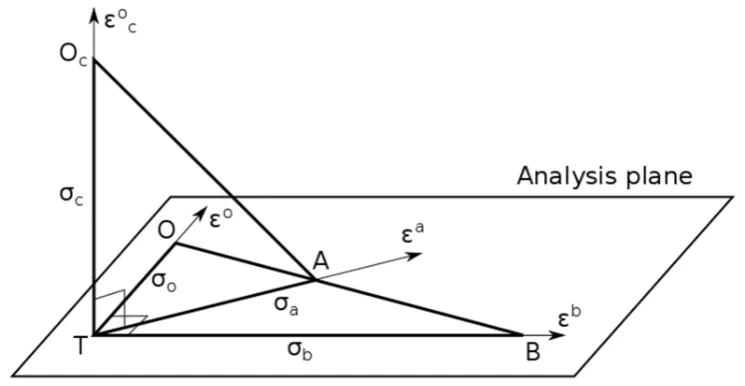
Figure 1 illustrates the statistical relationship in observation space between: the active observation
184
oy (illustrated as O in the figure), the prior or background yb (i.e. B), the analysis ya (i.e. A), and the
185
independent observation yc (i.e. Oc). The origin T corresponds to the truth of the scalar quantity,
186
and also corresponds to the zero of the central moment of each random variables, e.g. y−E[y], since
187
each variables are assumed to be unbiased. We also assume that the background, active and passive
188
observations errors are uncorrelated to one another, so the three axes; εo for the active observation
189
error, εb for the background error, and εco for the passive observation error are orthogonal. The
190
plane defined by εo and εb axes is the space where the analysis takes place, and is called the analysis
191
plane. But since we define the analysis to be linear and unbiased, only linear combinations of the form
192
b o
a ky k y
y = +(1− ) where k is a constant are allowed. The analysis A then lies on the line (B,O). The
193
thick lines in Figure 1 represent the norm of the associated error. For example, the thick line along the
194
oε axis depict the (active) observation standard deviation σo, and similarly for the other axes and
195
other random variables. Since the active observation error is uncorrelated with the background error,
196
the triangle ΔOTB is a right triangle, and by Pythagoras theorem we have,
197
2 2
2: ( ),( )
)
sum of background and observation error variances. The analysis is optimum when the analysis error
199
2 2 ||
||εa =σa is minimum, in which case the line (T,A)is perpendicular to line (O,B).
200
201
202
Figure 1. Hilbert space representation of a scalar analysis and cross-validation problem. The
203
arrows indicate the directions of variability of the random variables, and the plane defined by
204
the background and observation errors εb, εo defines the analysis plane. The thick lines
205
represent the norm associated with the different random variables. T indicate the truth, O the
206
active observation, B the background, A the analysis and Oc the passive observation.
207
208
Now let’s consider the passive observation Oc. The passive observation error is perpendicular to
209
the analysis plane, thus the triangle ΔOcTA is a right triangle,
210
2 2 2: ( ) ,( ) )
(yc−ya = O−A c O−A c =σc +σa, (17)
211
where σc2 is the passive observation error variance. The most important fact to stress here is that the
212
orthogonality expressed in eq.(17) is true whether or not the analysis is optimal. Furthermore, as the
213
distance (yc−ya)2 varies with the position of A along the line (O,B), the distance (yc−ya)2
214
reaches a minimum value when σa2 is minimum that is when the analysis is optimal. We thus also
215
argue from this representation that there is always a minimum, and the minimum is unique. Finally we
216
note that ΔBTOc is also a right triangle so that (yc−yb)2:= (O−B)c,(O−B)c =σc2+σb2, which is the
217
scalar version of eq.(9).
218
To extend this formalism to random vectors requires to define a proper matricial inner product as
219
briefly described in §1.2 of Caines [15]. It is important here to distinguish the stochastic metric space
220
from the observation vector space. In the stochastic metric space a “scalar” needs not to be a number,
221
but only a non-random quantity invariant with respect to E[]. Hence, we can define an Hilbert space
222
with the following (stochastic scalar) matricial inner product
223
) , cov( )] ) ( ))( ( [(
,w y y w w y w
y =E −E −E T = . The matrix nature of cov(y,w) pertains to the
224
observation vector space, but it remains a scalar with respect to the stochastic Hilbert space herein
225
defined. In order to obtain a true scalar (∈ R ), one would need to define a metric on the observation
226
space matrices as well, such as the trace. Also to be able to compare active and passive observations,
227
projectors need to be introduced on the observation space, implying yet another metric structure on the
228
observation space. We do not carry out this formalism here as it would represent a rather lengthy
229
development which would distract us from the main purpose of this paper; this will be considered in a
future manuscript. Finally, we remark that Hilbert space representation of random variables in infinite
231
dimensional space (i.e. continuous space) can also be defined, see Appendix 1 of Cohn [16].
232
2.4. Error covariance diagnostics in active observation space for optimal analysis
233
An analysis is optimal if the analysis error E[(εa)Tεa] is minimum. This implies that the gain
234
matrix using the prescribed error covariances, K~ in eq.(1), must be identical to the gain using the true
235
error covariances, i.e. K~=BHT(HBHT+R)−1 [7,8]. It is important to mention that necessary and
236
sufficient conditions to obtain the true error covariances in observation space that is HBHT and R,
237
are: 1 - the Kalman gain condition, HK~ =HKtrue and 2- the innovation covariance consistency,
238
R H B
H~ ~
] ) )(
[(O−B O−BT = T+
E . For a proof see the Theorem on error covariance estimates in Ménard [8].
239
From the optimality of the analysis (or Kalman gain) alone, we derive that E[(Aˆ−T)(O−B)T]=0
240
or E[(Aˆ−T)(O−Aˆ)T]=0. Indeed, from eq.(2), we get (O−Aˆ)=R(HBH+R)−1d, and for the analysis
241
error in observation space we get, (Aˆ−T)=R(HBHT +R)−1H
ε
f +HBHT(HBHT+R)−1ε
o, from which242
we derive the expectations above. Using the geometrical representation in §2.3 the distance between A
243
and T is minimum, when ΔTAO and ΔTAB (Figure 1) are right triangles. We should also note that for
244
the scalar problem, the Kalman gain depends only on the ratio of observation to background error
245
variances and thus the scalar Kalman gain is optimal if the ratio of the prescribed error variances is equal
246
to the ratio of the true error variances.
247
If in addition to the optimality of the analysis or Kalman gain we add the innovation covariance
248
consistency then we get three different statistical diagnostics of the (optimal) analysis error covariance.
249
Hollingsworth and Lönnberg [6] was the first to introduce a statistical diagnostic of analysis error in the
250
active observation space, as
251
T HL T
A O A
O ˆ)( ˆ) ] R HAˆ H
[( − − = −
E . (18)
252
Here we use a subscript, HL to indicate that this is the Hollingsworth-Lönnberg estimate. Eq.(18) can
253
obtained from the covariance of (O−Aˆ) and that, for an optimal gain matrix,
254
R R HBH R R H A
Hˆ T = − ( + )−1
which derives from the usual formula, Aˆ =B−BHT(HBH+R)−1HB.
255
Geometrically it derives from the fact that the triange ΔTAˆO is a right triangle, and from the
256
innovation covariance consistency that implies that the triangle ΔOTBis a right triangle. Using data to
257
construct E[(O−Aˆ)(O−Aˆ)T], an estimated analysis error covariance obtained from eq.(19) is symmetric
258
but could be non-positive definite as it is obtained by subtracting two positive definite matrices. The
259
effect of misspecification in the prescribed error covariances resulting from a lack of innovation
260
covariance consistency will be discussed in the result section §3 and in Appendix B.
261
Inspired from the geometrical interpretation that ΔTAB is also be a right triangle we derived the
262
following diagnostic,
263
T MDJ T
MDJ T
T
B A B
Aˆ )(ˆ ) ] HBH HAˆ H H(B Aˆ )H
[( − − = − = −
E , (19)
264
where MDJ stands for Ménard-Deshaies-Jacques. This relationship is obtained by using the expression
265
d R HBH
HBH ( ) 1
) ˆ
(A−B = T + −
, the innovation covariance consistency and the formula for the optimal
266
analysis error covariance Aˆ =B−BHT(HBH+R)−1HB. As for the HL diagnostics, the estimated error
267
covariance obtained from this diagnostic is symmetric by construction but may not be positive definite.
268
Another way of looking at eq.(19) is that it expresses, in observation space, the error reduction due to the
269
use of observations.
270
Another diagnostic of analysis error covariance was proposed by Desroziers et al. [7]. By
271
combining (O−Aˆ) and (Aˆ−B) we get
T D T
B A A
O ˆ)(ˆ ) ] HAˆ H
[( − − =
E , (20)
273
where the subscript D denotes the Desroziers et al. estimate. By construction, the estimated analysis
274
error covariance is not necessarily symmetric. A geometrical derivation is provided in Appendix A.
275
We also provide in Appendix B a sensitivity analysis on the departure from innovation covariance
276
consistency for each diagnostics, as well as for those in passive observation space which we we will for
277
for our discussion.
278
2.5. Error covariance diagnostics in passive observation space for optimal analysis
279
We can also derive optimal analysis diagnostics in the passive observation space. Considering the
280
3D geometric interpretation, and in particular the tetrahedron (Oc,T,A,B), we notice that since ΔTAB
281
is a right triangle, so is ΔOcAB, which is a projection of the triangle ΔTAB on the plane passing
282
through Oc, O and B. We thus have E[(Aˆ−B)c(Aˆ−B)Tc]+E[(O−Aˆ)c(O−Aˆ)Tc]= E[(O−B)c(O−B)Tc].
283
Combining this result with eq.(7) and using, E[(O−B)c(O−B)Tc]=HcBHcT+Rc, we then get
284
T c MDJ c T c c T c c A B
B
Aˆ ) (ˆ ) ] HBH H Aˆ H
[( − − = −
E . (21)
285
Note that our analysis diagnostic is the only diagnostic that is valid in both active and passive
286
observation spaces, i.e. eq.(21) is similar to eq.(19). The other, less direct, diagnostic for optimal
287
analysis is simply based on eq.(7) that is
288
T c c c c T
c c
Lc O A O A L
H A
H
R ˆ( , )
} ] ) ( ) [( { min arg
, γ
γ E − − = + . (22)
289
These five diagnostics will be used later in the results section .
290
3. Results with near optimal analyses
291
3.1. Experimental setup
292
We will just give here a short summary of the experimental setup we are using in this study. More
293
details can be found in the Part I paper (Ménard and Deshaies-Jacques [5]). A series of hourly analyses
294
of O3 and PM2.5 at 21 UTC for a period of 60 days (June 14 to August 12, 2014) were performed using an
295
optimum interpolation scheme combining the operational air quality model GEM-MACH forecast and
296
the real-time AirNow observations (see §2 of [5] for further details). The analyses are made off-line so
297
they are not used to initialize the model. As input error covariances, we use uniform observation and
298
background error variances, with R~=σo2I and B~=σb2C, where C is an homogeneous isotropic error
299
correlation based on a second-order autoregressive model. The correlation length is estimated by using
300
a maximum likelihood method using at first error variances obtained from a local
301
Hollingworth-Lönnberg fit [7] (and only for the purpose of obtaining a first estimate of the correlation
302
length). We then conduct a series of analyses by changing error variance ratio
γ
=σ
o2/σ
b2 while at the303
same time respecting the innovation variance consistency condition,
σ
o2+σ
b2=var(O−B). This304
corresponds basically in minimizing the tr (trace) of eq.(7) while the trace of the innovation covariance
305
consistency, tr[R+HBHT]=tr{E[(O−B)(O−B)T]}, is respected.
306
By leaving out 1/3rd of the observations for verification and constructing analyses with the
307
remaining 2/3rd, we construct a cross-validation setup from which we can evaluate the diagnostic
308
} ) ( ) [( { )
var( T
c c
c tr O A O A A
O− = E − − in passive observation space. This constitutes our first guess
309
experiment that we will refer to as iter 0. No observation or model bias was applied, and the
310
innovation mean at the station were removed prior to perform the analysis. The statistic are first
311
computed at the station using the 60-day members, and then was averaged over the domain so to give
the equivalent of a tr (trace). The mean value statistic for the three subsets are then averaged. More
313
details can be found in §2 and beginning of §3 of Part I [5].
314
The red curve on Figure 2 illustrates how this diagnostic varies with γ and exhibits a minimum.
315
This minimum can easily be understood by referring to Figure 1: as the analysis point A changes
316
position along the line (O,B) the distance Oc−A reaches a minimum, and this is what we observe in
317
Figure 2.
318
319
320
321
322
323
324
325
326
327
328
329
330
331
332
Figure 2. Variance of observation-minus-analysis of O3 in passive observation space. Red line,
333
and the variance of observation-minus-model, blue line.
334
335
In our next step, iter 1, we address the issue related to the spatial correlation that has not being
336
optimized. Our approach consist in using a variance estimator sequentially with a maximum
337
likelihood estimation of correlation length as was done in Ménard [8]. So, to refine our estimate of
338
model covariance in iter 1, we use the variances verifying the optimal ratio γˆ of iter 0 and the
339
innovation variance consistency to re-estimate by, maximum likelihood, the correlation length of C~ .
340
Then, in a procedure identical to iter 0 we estimate the optimal γˆ (iter 1) , which turn out to be very
341
close to the value obtained in iter 0. By innovation variance consistency we thus get improved
342
estimates for the observation and background error variances, from which we will compute a number of
343
statistical diagnostics of the analysis error variance in the section that follows. However, as before, we
344
do not attempt to provide a spatial distribution of the error statistics that are still assumed uniform. A
345
summary of the main features of the two experiments are presented in Table 1. The χ2/Ns value
346
shown in Table 1 is the 60-day mean value of χk2/Ns(k) where Ns(k) is the total number of
347
observations available at time tk . We observe that there was a significant improvement from iter 0 to
348
iter 1 in terms of χ2/Ns but is still not equal to one. We thus refer the analysis of iter 1 as near
349
optimal.
350
351
Table1. Input error statistics for the first experiment and optimized variance ratio experiment
352
Experiment
Lc(km)
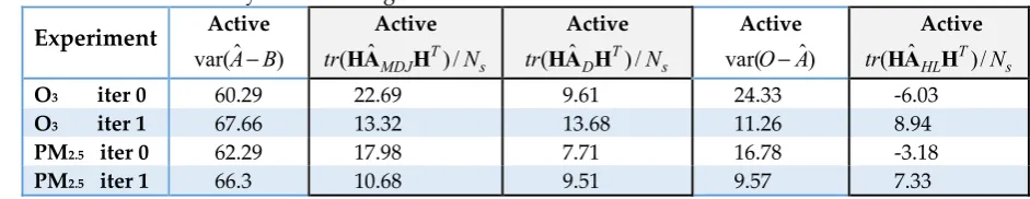
(O−B)2 γ =ˆ σˆo2/σˆb2 σˆo2 σˆb2 χ2/NsO3 iter 0 124 101.25 0.22 18.3 83 2.23
O3 iter 1 45 101.25 0.25 20.2 81 1.36
PM2.5 iter 0 196 93.93 0.17 13.6 80.3 2.04
353
This procedure converges really fast and in practice there is no need to go beyond iter 1. Figure 3
354
displays iterates 0 to 4 with our estimation procedure for O3. With one iteration update we nearly
355
converge. A similar procedure was used in Ménard [8], where the variance and correlation length
356
(estimated by maximum likelihood) were estimated in sequence, which taught us that a slow and
357
fictitious drift in estimated variances and correlation length can occur when the correlation model is not
358
the true
359
360
Figure 3. Optimal estimates of σo2, σb2 and maximum likelihood estimate of correlation
361
length Lc for the first four iterates. Blue, is the optimal background error variance, green, the
362
optimal observation error variance and in red the correlation length (in km, with labels on the
363
right side of the figure).
364
365
correlation. So in regard of similar considerations that may occur here, we do not extend our iteration
366
procedure beyond the first iterate.
367
3.2. Statistical diagnostics of analysis error variance
368
For each of these experiments statistics related diagnostics for analysis error variance, discussed in
369
§2, are computed and the results are presented in Table 2 for the verification made against active
370
observations, and in Table 3 to the verification made against the passive observations.
371
372
Table2. Analysis statistics against active observations
373
Experiment
Active) ˆ var(A−B
Active
s T MDJ N
tr(HAˆ H )/
Active
s T D N
tr(HAˆ H )/
Active ) ˆ var(O−A
Active
s T HL N
tr(HAˆ H )/
O3 iter 0 60.29 22.69 9.61 24.33 -6.03
O3 iter 1 67.66 13.32 13.68 11.26 8.94
PM2.5 iter 0 62.29 17.98 7.71 16.78 -3.18
PM2.5 iter 1 66.3 10.68 9.51 9.57 7.33
374
The second, third and last column of Table 2 are tabulated estimates of the analysis error variance at
375
the active location sites, i.e. tr(HAHT)/Ns, obtained by three different methods. The second column is
376
an estimate given with our method
σ
b2−var(Aˆ−B)=tr(HAˆMDJHT)/Ns . The third column is the377
Desroziers et al. estimate of analysis error [7], eq.(20), and the last column is the estimate using the
378
method proposed by Hollingsworth and Lönnberg [6], eq.(18). We note that the analysis error variance
379
estimate provided by the first two methods is fairly consistent for an updated correlation length
estimate, i.e. iter1 (but not iter0). We also note that χ2/p is closer to one for iter1. These two facts
381
indicate that the updated correlation length (iter1) with uniform error variances is closer to the
382
innovation covariance consistency. The Hollingsworth and Lönnberg [6] method however, is very
383
sensitive and negatively biased in the lack of innovation covariance consistency.
384
Estimate of the analysis error variance at the passive observation locations, i.e. tr(HcAHTc)/Ns ,
385
provided by two different methods are given by eq.(21) in column 3 and by eq.(22) in column 5 of table
386
3. As for the estimate at the active locations (Table 2), there is a general agreement on the analysis error
387
estimates with the updated correlation length (iter1), although this distinction is not that clear for PM2.5.
388
389
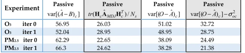
Table3. Analysis statistics against passive observations
390
Experiment
Passive] ) ˆ var[(A−B c
Passive
s T c MDJ
c N
tr(H Aˆ H )/
Passive ] ) ˆ var[(O−Ac
Passive 2 ] ) ˆ
var[(O−Ac −
σ
ocO3 iter 0 56.95 26.03 51.02 32.72
O3 iter 1 52.04 28.95 48.95 28.75
PM2.5 iter 0 62.29 22.65 38.09 24.49
PM2.5 iter 1 66.3 24.62 38.28 21.38
391
We note also that the analysis error variance at the active sites is smaller than the analysis error
392
variance at the passive observation sites. This involves in particular the fact that since the passive
393
observation are away from the active observation sites, the reduction of variance at the passive
394
observation sites is smaller than at the active observation sites.
395
3.3. Comparison with the perceived analysis error variance
396
We computed the analysis error covariance A resulting from the analysis scheme, the so-called
397
perceived analysis covariance [9], using the expression,
398
T T HBH R HB B GG
H B B
A=~−~ ( ~ +~)−1 ~=~− . (23)
399
We then compared the perceived analysis error variance with the estimated active analysis error
400
variance from the previous subsection.
401
402
Figure 4. Analysis error variance for ozone optimal analysis case O3 iter1. Left panel is the
403
analysis error on the model grid and on the right panel at the active observation sites. Note
404
that the color bar of the left and right panels are different. The maximum of the color bar for
405
407
In order to calculate the perceived analysis error covariance eq.(23) we first perform a Choleski
408
decomposition of HB~HT +R~=LLT, where L is a lower triangular matrix. Then with a forward
409
substitution we obtain L−1, from which we compute G=B~HTL−T. The perceived analysis error
410
variance for the ozone optimal analysis (i.e. O3 iter1) is displayed in Figure 4 (A similar figure but for
411
PM2.5 is given in supplementary material). We note that although the input statistics used for the
412
analysis are uniform (i.e. uniform background and observation error variances, and homogeneous
413
correlation model), the computed analysis error variance at the active observation location displays
414
large variations, which is attributed to the non-uniform spatial distribution of the active observations.
415
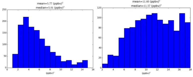
In Figure 5 we display a histogram of those variances for the ozone optimal analysis O3 iter1 (right
416
panel) and for the first experiment O3 iter0 (left panel) without optimization (A similar figure is but for
417
PM2.5 is given in supplementary material). Note that median or mean values of variances are
418
significantly different between the optimal and non-optimal analysis cases. We also observe two
419
maxima, one of which is actually due to isolated observation sites. At those sites the analysis error
420
variance is simply obtained by the scalar equation 1/σa2= 1/σo2 +1/σb2. For O3 iter1 the scalar
421
analysis error variance gives 16.2, and for O3 iter0 we get 15.0, thus explaining the secondary maxima.
422
423
424
Figure 5. Distribution (histogram) of the ozone analysis error variance at the active
425
observation locations. First analysis experiment O3 iter0 (no optimization) on the left panel,
426
and optimal analysis case O3 iter1 on the right panel.
427
428
The mean perceived analysis error variance for all experiments is presented in Table 4.
429
Comparing these values with the estimated values of analysis error variance based on diagnostics in
430
Table 2 we note that for both optimal experiments, O3 iter1 and PM2.5 iter1, the perceived analysis error
431
variance roughly agrees with all analysis error variances estimated with diagnostics (Table 2). But for
432
the non-optimal analyses, O3 iter0 and PM2.5 iter0, there is a general disagreement between all
433
estimated values.
434
435
Table 4. Perceived analysis error variance. Mean over active observation sites.
436
Experiment
Perceiveds T P N
tr(HA H )/ O3 iter 0 5.77
Looking more closely, however, we note that the agreement in the optimal case is not perfect. The
437
perceived analysis error variance is about 20% lower than the best estimates tr(HAˆMDJHT)/Ns and
438
s T
D N
tr(HAˆ H )/ . The optimal χ2/Ns values in the “optimal” cases are slightly above one, thus
439
indicating that some more tuning of the error statistics could be done to between reach an innovation
440
consistency. More on that matter will be presented in §4.5.
441
4. Discussion on the statistical assumptions and practical applications
442
4.1 Representativeness error with in situ observations
443
The statistical diagnostics presented in §2 derive from the assumption that the observation errors
444
are horizontally uncorrelated and uncorrelated with the background error. Although this assumption
445
is never entirely observed in reality, there are ways to work around it. In the case of in situ
446
observations, and assuming that any systematic error have been removed, random errors are still
447
present, due to the difference between the observation and the model’s equivalent of the observation –
448
called representativeness error (see Janjic et al. [18] for a review). Representativeness error is due to
449
unresolved scales and processes in the model and interpolation or forward observation model errors.
450
These errors are typically roughly at the scale of the model grid [19,20], so typically a few tens of
451
kilometers for air quality models. This should not be confused with the representativeness of an
452
observation, where, for example, remote stations are representative of large area (e.g. several hundreds
453
of kilometers), whereas urban and suburban stations are at the scale of human activity in the cities,
454
traffic and industries, etc. and are, depending on the chemical specie, of a few kilometers and less.
455
Representativeness error of in situ measurements can be discarded altogether by simply filtering
456
any pair of observations that are in the range of a few model grid size, both in assimilation and
457
estimation of error statistics [1] or in pairs of passive-active observations for cross-validation [12]. Once
458
this filtering is done, the assumption on observation errors being spatially uncorrelated and
459
uncorrelated with the background error then applies.
460
4.2 Correlated observation-background errors
461
In any case, it is interesting to show how the different diagnostics, introduced in §2, depends on the
462
statistical assumptions of the observation error. One way to get an understanding of the effect of these
463
assumptions is to look at it from a geometrical point of view, using the representation introduced in §2.2.
464
Note that the same results can be obtained analytically, but the geometrical interpretation gives a simple
465
and appealing way of looking at the problem.
466
Let us consider the effect on the analysis of observation error correlated with background error.
467
The case were the observation error is uncorrelated with background error is represented in Figure 6 on
468
the left panel and when we they are correlated on the right panel. The observation and background
469
error variances are kept unchanged, with the same (O,T) length and (B,T) length in both panels. In
470
the case of correlated errors the angle ∠BTO is no longer a right angle. Yet, it is still possible to obtain
471
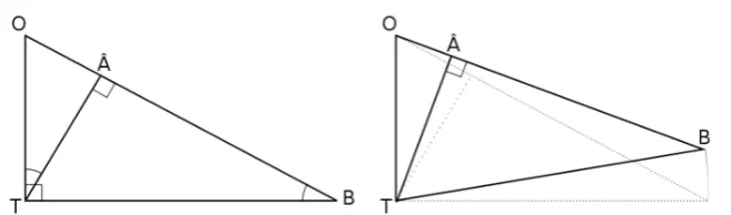
an optimal analysis, Aˆ , as a linear
474
Figure 6. Geometrical representation of the analysis. Left panel, for observation errors
475
uncorrelated with the background error. Right panel, with correlated errors. T indicate the
476
truth, O the observation, B the background and Aˆ the optimal analysis.
477
478
combination of the observation and the background, on the line (O,B), for which the distance Aˆ to T
479
(i.e. the analysis error variance) is minimum. In this case, (Aˆ ,T)⊥(O,B). Note that for strongly
480
correlated errors and when σ >b2 σo2, although Aˆ is still on the line (O,B), it may actually lie outside
481
the segment [O,B]. Yet, the principles and theory still hold in that case.
482
When the observation error is uncorrelated with the background error, (O ,T)⊥(B,T) , the
483
triangles ΔOTAˆ and ΔTBAˆ are similar and it follows that (O−Aˆ)(Aˆ−B) = (Aˆ−T)2, which is the
484
Desroziers et al. [7] diagnostic for analysis error variance. But, when the observation error is correlated
485
with the background error (right panel of Figure 6), the triangles ΔOTAˆ and ΔTBAˆ are no longer
486
similar triangles and the Desroziers et al. [7] diagnostics for analysis error does not hold (see derivation
487
in Appendix A). However, the HL, eq.(18), and MDJ diagnostic, eq.(19), depend only on having right
488
triangles ΔOTAˆ and ΔTBAˆ , and not on the orthogonality of (B,T)with (O,T). Therefore, the HL
489
and MDJ diagnostics are valid with or without correlated observation-background errors.
490
4.3 Estimation of satellite observation errors with in situ observation cross-validation
491
One of the important problems in satellite assimilation is the estimation of the satellite observation
492
error, which could be addressed with a simple modification of our cross-validation procedure. Let us
493
assume that we have in situ observations that we assume to have uncorrelated errors between
494
themselves (or use a filter with a minimum distance as discussed in §4.1), with the background errors
495
and the satellite observation errors. Yet, the satellite observation errors could be correlated with the
496
background error. Satellite observations could come from a multi-channel instrument with
497
channel-correlated observation errors, as found with many instruments, and yet our validation
498
procedure can still be used. Let us consider that the analyses comprise of satellite and in situ
499
observations but, for the purpose of cross-validation, we use only 2/3rd of the in situ observations in the
500
analysis, and keep the remaining 1/3rd as passive to carry out the cross-validation procedure.
501
The first thing to note is that the passive in situ observations have uncorrelated errors with the
502
analysis error (the analysis is composed of satellite observations and 2/3rd of the in situ observations).
503
We then use eq.(7) where the interpolation of the analysis is made only at the in situ active observations.
504
Minimizing E[(O−A)Tc(O−A)] (i.e. the trace of the l.h.s.of eq.(7)) results in finding the optimal in situ
505
observation weight. Then, computing the analysis error covariance in the satellite observation space
506
from the analysis scheme (either from a Hessian of a variational cost function, or with an explicit gain as
507
in eq.(23)), i.e. HsatAˆHTsat , we use the HL formulation eq.(18) to obtain the satellite observation error
508
covariance,
509
sat T
sat sat
T sat
satAH O A O A R
H ˆ + e[( − ) ( − ) ]= . (24)
The equation (24) has the important properties that the estimated observation error covariance is
511
symmetric and positive definite by construction. Then, a new analysis could be carried out to obtain a
512
more realistic HsatAˆHTsat, with a resulting updated Rsat, and so forth until convergence.
513
4.4 Remark on cross-validation of satellite retrievals
514
As a last remark, it appears that cross-validation of satellite retrieval observations using a k-fold
515
approach where the observations are used as passive observations to validate the analysis can be a
516
difficult problem. Retrievals from passive remote sensing at nadir generally involve a prior or
517
climatology or a model assumption over different regions, and is thus likely to have spatially correlated
518
errors and errors correlated with the background error. It doesn’t mean, however, that nothing can be
519
done in that case. For example, for certain sensors, such as infrared sensors, it is possible to disentangle
520
the prior from the retrieval, so that by an appropriate transformation of the measurements, observations
521
can be practically decorrelated from the background [21,22]. However to the authors’ knowledge, such
522
an approach have never been undertaken for visible measurements such as for NO2 or AOD’s.
523
4.5 Lack of innovation covariance consistency and its relevance to the statistical diagnostics
524
The error covariance diagnostics for optimal analysis, presented in §2.4 and §2.5, depends on the
525
innovation covariance consistency, E[(O−B)(O−B)T]=HB~HT+R~ , and our results presented in §4
526
have shown that the different estimates for the optimal analysis error variance are close, but do not
527
strictly agreeing to each other. This disagrement is related to the lack of innovation consistency as
528
follows.
529
Let us introduce a departure matrix Δ from innovation covariance consistency as,
530
Δ + = +R − I
H B H d
d ]( ~ ~) 1
[ T T
E . (25)
531
The trace of eq.(25), which is related to χ2, is given by
532
Δ) ( }
) ~ ~ ( ] [ { ]
[ 2 =tr EddT HBHT+R −1 = Ns+tr
E
χ
. (26)533
We recall that in the experiment iter 1 we got χ2/Ns values of 1.36 for O3 and 1.25 for PM2.5 (see Table
534
1), indicating that the innovation covariance consistency is deficient, although less serious than with the
535
experiment iter 0 where values of 2 and higher have been obtained.
536
If we take into account the fact that there can be a difference between E[ddT] and (H~BHT+R~)
537
and we rederive the (active) analysis error covariance for HL, MDJ and D schemes, we get (see Appendix
538
B)
539
} {
} ~ { } ~ { } ˆ { } ˆ
{ T true T MDJ
HL tr tr tr tr
tr HA H = HA H + RΔ − HBHTΔ + error (27)
540
} {
} ˆ { } ˆ
{ MDJ T tr true T tr MDJ
tr HA H = HA H − error (28)
541
} { } ˆ { } ˆ
{ D T tr true T tr D
tr HA H = HA H − error , (29)
542
where tr{errorMDJ}=tr{(HB~HT)(HB~HT+R~)−1Δ(HB~HT)} , { } {~( ~ T ~) 1 ( ~ T)} D tr
tr error = R HBH +R − Δ HBH .
543
We note that although the error terms are complex expressions, they all depend linearly on Δ. Thus,
544
the disagreement between the HL, MDJ and D analysis error variance estimates is due to lack of
545
innovation covariance consistency.