arXiv:astro-ph/0307104v2 29 Aug 2003
Large Scale Cosmic Microwave Background Anisotropies
and Dark Energy
J. Weller
1⋆and A.M. Lewis
21Institute of Astronomy, University of Cambridge, Madingley Road, Cambridge CB3 0HA. 2CITA, 60 St. George St, Toronto M5S 3H8, ON, Canada
Accepted ???, Received ???; in original form 2 February 2008
ABSTRACT
In this note we investigate the effects of perturbations in a dark energy component with a constant equation of state on large scale cosmic microwave background anisotropies. The inclusion of perturbations increases the large scale power. We investigate more speculative dark energy models withw <−1 and find the opposite behaviour. Overall
the inclusion of perturbations in the dark energy component increases the degenera-cies. We generalise the parameterization of the dark energy fluctuations to allow for an arbitrary constant sound speeds and show how constraints from cosmic microwave background experiments change if this is included. Combining cosmic microwave back-ground with large scale structure, Hubble parameter and Supernovae observations we obtain w =−1.02±0.16 (1σ) as a constraint on the equation of state, which is
al-most independent of the sound speed chosen. With the presented analysis we find no significant constraint on the constant speed of sound of the dark energy component.
Key words: cosmology:observations – cosmology:theory – cosmic microwave back-ground – dark energy
1 INTRODUCTION
Observations of distant supernovae give strong indica-tions that the expansion of the universe is accelerating (Perlmutter et al. 1997; Riess et al. 1998; Perlmutter et al. 1999; Riess et al. 2001). This is consistent with various other evidence, including recent precision observations of the cos-mic cos-microwave background (Spergel et al. 2003). These ob-servations can in principle be explained by a cosmologi-cal constant term in Einstein’s equation of gravity. How-ever, all that is really required to obtain accelerated expan-sion of the universe is the existence of a fluid component which dominates the universe today and which has a ra-tio of pressure to energy density of w ≡ pde/ρde <−1/3. Quintessence models, which assume a scalar field as the dark energy component (Wetterich 1988; Ratra & Peebles 1988; Peebles & Ratra 1988), differ from a cosmological constant model in that the equation of state parameter is not neces-sarily w =−1, and may be evolving. Furthermore a dark energy fluid withw6=−1 will have perturbations.
In light of the recent cosmic microwave background (CMB) data of the Wilkinson Microwave Anisotropy Probe (WMAP) (Hinshaw et al. 2003) we re-investigate the con-straints on a dark energy component with a constant equa-tion of state and stress the importance of including
pertur-⋆ Email: J.Weller@ast.cam.ac.uk
bation in the dark energy. We note that perturbations have been included in the analysis of the WMAP team.
If the dark energy is not a cosmological constant, gen-eral relativity predicts that there will be perturbations. Even if dark energy is expected to be relatively smooth, for a con-sistent description of CMB perturbations it is necessary to include perturbations in the dark energy (Coble et al. 1997; Viana & Liddle 1998; Caldwell et al. 1998; Ferreira & Joyce 1998). We also allow for models with w < −1, as sug-gested by Caldwell (2002). These models might be real-ized in non-minimally coupled scalar field dark energy mod-els (Amendola 1999; Boisseau et al. 2000) or k-essence with non-canonical kinetic terms (Armendariz-Picon et al. 2000). Although the stability of such models is hard to achieve (Carroll et al. 2003), from an observational point of view one should not rule out the possibility in advance. Recent constraints from x-ray and type Ia Supernovae observation have constrained the equation of state tow=−0.95±0.30 ( Schuecker et al. 2003).
2 LARGE SCALE COSMIC MICROWAVE ANISOTROPIES
We will concentrate in this analysis on the behaviour of the temperature anisotropy power spectrum given by the covari-ance of the temperature fluctuation expanded in spherical harmonics
Cl= 4π
Z
dk
k Pχ|∆l(k, η0)|
2. (1)
∆l(k, η0, µ) gives the transfer function for eachℓ,Pχ is the initial power spectrum andη0 is the conformal time today. On large scales the transfer functions are of the form
∆l(k, η0) = ∆LSSl (k) + ∆ISWl (k), (2) where ∆LSSl (k) are the contributions from the last scatter-ing surface given by the ordinary Sachs-Wolfe effect and the temperature anisotropy, and ∆ISWl (k) is the contribu-tion due to the change in the potentialφ along the line of sight and is called the integrated Sachs-Wolfe (ISW) effect. The ISW contribution can be written (Sachs & Wolfe 1967; Hu & Sugiyama 1995)
∆ISWl (k) = 2
Z
dηe−τ(η)φ′j
l[k(η−η0)]
whereτ(η) is the optical depth due to scattering of the pho-tons along the line of sight, jl(x) are the spherical Bessel functions, and the dash denotes the derivative with respect to conformal timeη. The frame-invariant potentialφcan be defined in terms of the Weyl tensor, and is equivalent to the Newtonian potential in the absence of anisotropic stress (see Challinor & Lasenby (1999) for an overview of the covariant perturbation formalism we use here).
The Poisson equation relates the potential to the den-sity perturbations via
k2φ=−4πGa2δρ , (3) where δρis the total comoving density perturbation. Thus the source term for the ISW contribution assuming only matter and dark energy is given by
k2φ′=−4πG ∂
∂η
a2(δρm+δρde) , (4)
where the perturbations are evaluated in the rest frame of the total energy. The magnitude of the ISW contribution therefore depends on the late time evolution of the total density perturbation.
In general the fractional perturbationsδi≡δρi/ρiof a non-interacting fluid evolve as
δ′
i+ 3H(c2s,i−wi)δi+ (1 +wi)kvi=−3(1 +wi)h′, (5) whereHis the conformal Hubble parameter,viis the veloc-ity,wi≡pi/ρi, andh′= (δa/a)′, where the local scale factor
ais defined by integrating the Hubble expansion. The sound speedc2s is frame-dependent, and defined asc2s≡δp/δρ.
Neglecting anisotropic stress the potentialφevolves as
φ′′+ 3H(1 +p′
ρ′)φ ′+k2p′
ρ′φ+
(1 + 3p ′
ρ′)H 2+ 2H′
φ
= 4πGa2(δp−p
′
ρ′δρ), (6)
where the RHS is a frame invariant combination. For a con-stant total equation of state parameterwtotthis becomes
φ′′+ 3H(1 +w
tot)φ′= 4πGa2δp. (7)
In matter or cosmological constant domination the comov-ing pressure perturbation is zero on scales where the baryon pressure is negligible. In this case the growing mode is the solutionφ= const, and there is no contribution to the ISW effect. However for varyingwtot, as between matter and dark energy domination, or when there are dark energy pertur-bations, the potential will not be constant.
In general the evolution of the perturbations can be computed numerically. For a non-interacting fluid with con-stantwi, defining the frame invariant quantity ˆc2s,i(the fluid sound speed in the frame comoving with the fluid) we have the evolution equations
δ′
i+ 3H(ˆc2s,i−wi)(δi+ 3H(1 +wi)vi/k) +
(1 +wi)kvi=−3(1 +wi)h′ (8)
v′
i+H(1−3ˆc2s,i)vi+kA=kcˆ2s,iδi/(1 +wi), (9) where A is the acceleration (A = 0 in the vm = 0 frame (synchronous gauge),A=−Ψ in the zero shear frame (New-tonian gauge)). We have assumed zero anisotropic stress, which is the case for matter and simple dark energy models. Also note that a varying equation of state factor will lead to extra contributions to the ISW effect (Corasaniti et al. 2003).
2.1 Scalar Field Dark Energy
In order to study the full evolution of the dark energy fluid including fluctuations we need to specify the speed of sound and hence its density and pressure perturbations. A simple way to achieve this, is by relating the dark energy to a scalar field. In order to be able to analyse models with an equa-tion of statew >−1 as well asw <−1 we start with the Lagrangian (Carroll et al. 2003)
Lde=± 1 2(∂µϕ)
2
−V(ϕ), (10)
where the positive sign in front of the kinetic term corre-sponds tow >−1 solutions and the negative sign tow <−1,
ρde=± 1 2ϕ˙
2+V , p de=±
1 2ϕ˙
2−V , (11)
and dots denote normal time derivatives. The equations for the perturbations are therefore
δρde = ±ϕ˙(δϕ˙ ) +V,ϕδϕ±Aϕ˙2 (12)
δpde = ±ϕ˙(δϕ˙ )−V,ϕδϕ±Aϕ˙2 (13) whereAis the acceleration. In the frame in which the scalar field is unperturbed (the frame comoving with the dark en-ergy, denoted by a hat),cδϕ= 0 and so ˆc2
s≡δp/b δρb = 1. If the equation of state pde = wρde is constant, the dark energy density evolves like ρde = ρde,0 a−3(1+w). We can then identify this solution with a scalar field and its potential
V(ϕ) ≡ 1−w
2 ρde, (14)
˙
10−4 10−3 10−2 −0.01
0 0.01 0.02 0.03 0.04 0.05 0.06 0.07 0.08
k / Mpc−1
∆2
ISW
(k)
Figure 1.The quadrupole (l= 2) contribution to the integrated Sachs-Wolfe effect. The solid line is for a ΛCDM universe, the dot dashed line for a universe withw=−2 and the dashed line for w = −0.6. For the other cosmological parameters see text. The bold lines are including perturbations in the dark energy component and the thin lines excluding them.
Clearly a constant equation of state makes a very unnatu-ral quintessence model. However a large class of models are expected to be well described (at least as far as the CMB anisotropy is concerned) by an effective constant equation of state parameter. In this paper we do not explicitly consider dark energy models with an evolving equation of state.
In order to analyse the impact of the equation of state parameter of the dark energy component on the cosmic mi-crowave background anisotropies we will first look into pri-mary degeneracies originating from smaller scales in the temperature anisotropy power spectrum. As discussed in Melchiorri et al. (2002) the main impact is due to the change in the angular diameter distance toward the last scattering surface. The small scale CMB anisotropies in a flat uni-verse are mainly sensitive to the physical cold dark mat-ter and baryon densities and the angular diamemat-ter distance
dA ∝
R
[Ωm(1 +z)3+ Ωde(1 +z)3(1+w)]−1/2. Hence if w is decreasing, we need to increase Ωde and for a flat universe decrease Ωm and therefore increase the Hubble parameter
H0 and therefore decrease Ωb in order to obtain the same CMB anisotropy power spectrum.
Let us assume that we can by some artificial mecha-nism suppress the fluctuations in the dark energy compo-nent. Note that in general this is not consistent with the equations of general relativity. Only in the case of a cos-mological constant with w=−1 we recognise from Eqn. 5 that δρde = 0 is a solution. We implement the equations in the frame comoving with the dark matter (synchronous gauge), and allow for a changing background equation of state but fix the dark energy perturbations to zero. We com-pare results from applying this (incorrect) recipe with those obtained using the full equations consistent with linear gen-eral relativity. In their rest frame the matter perturbations evolve like
δ′′
m+Hδm′ = 4πGa2ρmδm (forcedδde= 0), (16)
Figure 2.CMB angular power spectra for different dark energy models with no perturbations. The solid line is for a ΛCDM model, the dotted line for a model withw =−0.6 and dashed linew=−2.0. The parameters Ωc, Ωb andH0 are adjusted to show the degeneracies as mentioned in the text.
which for matter domination (w = 0) results inδm∝a. If we gradually decreasewstarting fromw= 0, the transition between matter and dark energy domination happens later and later, but more and more rapidly, and with a larger over-all change in the equation of state. So we expect a smover-aller contribution to the ISW for values ofwcloser to zero.
In Fig. 1 we show the quadrupole contribution ∆ISW 2 (k) to the ISW. The solid line is for a ΛCDM universe with
w = −1, Ωm = 0.3, Ωb = 0.05, H0 = 65 km s−1Mpc−1, the thin dashed line is for w = −0.6, Ωm = 0.44, Ωb = 0.073, H0 = 54 km s−1Mpc−1 and the thin dot-dashed for
w=−2, Ωm= 0.17, Ωb = 0.027, H0 = 84 km s−1Mpc−1. For all three models the spectral index is fixed tons = 1.0 and the redshift of instantaneous complete reionization is
zre= 17. Without dark energy perturbations we clearly see that forw=−0.6 there is only a small contribution to the quadrupole from the ISW, while there is a large contribution forw=−2.
In the case of no dark energy perturbations for w = −0.6 there is a smaller ISW contribution than for a ΛCDM universe, and subsequently forw=−2 a larger ISW contri-bution. In Fig. 2 we show the entire temperature anisotropy power spectrum for the three degenerate models. We can see the increase in power on large scales by moving from the w = −0.6 over the w = −1 (ΛCDM) to the w = −2 model. If these were the true signatures of dark energy mod-els on large scales we might be hopeful that by cross correlat-ing large scale CMB anisotropies with x-ray or radio source power spectra (Boughn & Crittenden 2003) one could break the angular diameter distance degeneracy of the small scale anisotropies.
Figure 3. CMB angular power spectra for them dark energy models as in Fig. 2, butwithdark energy perturbations.
Hence the dark energy perturbations are anti-correlated with the matter perturbations as they are sourced.
The bold lines in Fig. 1 correspond to the case which includes perturbations. Note that for w=−1, the pertur-bations are exactly zero. We see how the bold dot-dashed line (w=−2) is significantly lowered compared to the thin line, due to the contribution of the perturbationδρde, while for w=−0.6 (dashed line) the contribution is significantly enhanced.
In Fig. 3 we show the CMB temperature anisotropy spectrum for the three models this time including perturba-tions. We clearly see that the large differences obtained on large scales when we didnotinclude perturbations in Fig. 2 have vanished. This is because forw >−1 the smaller over-all change in the background equation of state is enhanced by the contribution due to the perturbations in the dark energy component. Forw <−1 the large contribution from the different evolution of the background via the matter per-turbations is partially cancelled by the contribution of the dark energy fluctuation. It seems difficult to obtain informa-tion about the nature of dark energy from large scale CMB information.
2.2 Generalised Dark Energy Perturbations
We turn now to the problem of how to describe dark en-ergy perturbations without resolving to a scalar field. We should note as a reminder that we only resolved to a scalar field in order to have a prescription for calculating the per-turbations, where we assumed the most simple kinetic term ±(∂uϕ)2. These models have a speed of sound ˆc2s= 1. How-ever we have no idea what the dark energy actually is, so this assumption may be premature. For example, in a more generic class of dark energy models, so called k-essence, the kinetic term does not need to be of such a simple form (Armendariz-Picon et al. 2000) and the sound speed gen-erally differs from one. In the most general case the speed of soundandthe equation of state evolve with time, though clearly accounting for this is not feasible in general for
pa-102 103 104
10−8 10−6 10−4 10−2 100 102
η / Mpc
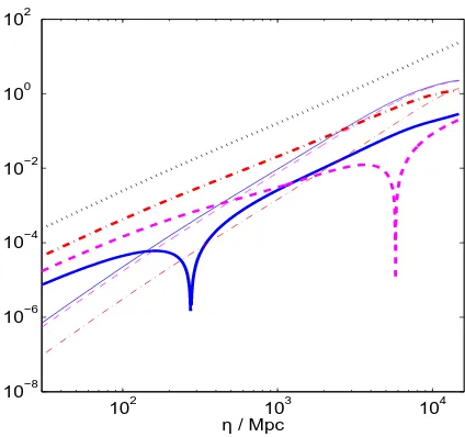
Figure 4.Evolution of|δde|(thick) andvde(thin) in the frame comoving with the dark matter perturbation (dotted line), for
w=−0.6 and ˆc2
s ={1,0.7,0.1} (solid, dashed and dash-dotted lines), andk= 10−3Mpc−1. Note that we plot the absolute val-ues of the fluctuations with amplitude normalized to unit initial curvature perturbation.
rameter estimation. Here we generalise the dark energy pa-rameterisation by introducing a constant sound speed ˆc2
s as a free parameter.
If δde is initially zero, we see from Eqn. 8 that it is sourced by the other perturbations ifw6=−1 via the time evolution of the local scale factor, the source term 3(1+w)h′. An over density causes a decrease in the local expansion rate and so h′ <0. In this case a fluid starts to fall into over-densities ifwi>−1, but starts to fall out if wi<−1. The subsequent evolution depends on the sound speed, as shown in Fig. 4. Consider the frame comoving with the dark mat-ter (whereA= 0). Whenk≪ Hthe term (1 +wi)kvi can be neglected, then the velocity and wavenumber only enter via the combination (1 +wi)vi/k. For large sound speeds the source term for the velocities is large and they are anti-damped, which leads to an almostk-independent evolution where the dark energy perturbations change sign at early times, and become theopposite sign to δm. At late times when the dark energy becomes a significant fraction of the energy density, the total density perturbations are there-fore smaller than without dark energy perturbations, there is a larger overal change in the potential, and the ISW con-tribution is increased. The sign reversal happens later for lower sound speeds as we see in Fig. 4 and for ˆc2
s∼1/3 the perturbations never reverse. Thus the contribution to the ISW effect from the perturbations decreases with the sound speed. Forw <−1 the effect is reversed, with the perturba-tions initially of opposite sign, and the contribution to the ISW effect increasing as the sound speed is decreased.
In Fig. 5 we show how the CMB temperature anisotropies change on large scales, for different constant ˆc2
s. We see that if we decrease the sound speed gradually from ˆ
c2
correlat-Figure 5.On the left the CMB anisotropies for thew=−0.6 model. The top solid line is with perturbations and the low dashed line for no perturbations. In between the speed of sound is decreasing from top to down withc2s= 0.2,0.05,0.01,0.0. On the right the CMB anisotropies for thew=−2.0 model. The lower solid line is with perturbations and the top dashed line for no perturbations. In between the speed of sound is increasing from top to down withc2s= 0.0,0.01,0.05,0.2. The thin dotted lines above (forw=−0.6) and below (forw=−2) correspond to sound speeds ofc2s= 5.0. Note that in both cases thatc2s= 1.0 corresponds to the solid line.
ing the large scale CMB power spectrum with direct mea-sures of the potential (Boughn & Crittenden 2003) might be an excellent probe for the sound speed of the dark energy component, if the equation of state is different fromw=−1.
3 PARAMETER CONSTRAINTS
In order to stress the importance of the inclusion of dark energy perturbations we will discuss their impact on the parameter estimation with CMB data. We included the per-turbations into the camb1 code (Lewis et al. 2000) (based
oncmbfast(Seljak & Zaldarriaga 1996)) and performed a
Markov-chain Monte Carlo parameter analysis using cos-momc2 (Lewis & Bridle 2002). We varied six non-dark
en-ergy cosmological parameters with flat priors: the baryon density Ωbh2, the cold dark matter density Ωch2, the ratio of the sound horizon to the angular diameter distance at last scatteringθ, the damping of the small scale CMB power due to reionizationZ ≡e−2τ(we assumeτ <0.3), the amplitude of the fluctuationsAsand the spectral index of the primor-dial power spectrumns. In addition we varied the constant equation of state parameter of the dark energy component
w, and where required the constant sound speed parameter in the range−3<log10ˆc2
s <2. The Hubble parameterH0 is derived from θ (Kosowsky et al. 2002), and the dark en-ergy density from the requirement that the background uni-verse is spatially flat. We assume negligible primordial tensor modes and neutrino mass, and include priors on the Hubble parameter from the Hubble Key project (Freedman et al. 2001), withH0= (72±8) km s−1Mpc−1, and a weak prior Ωbh2 = 0.022±0.002 (1σ) from Big Bang nucleosynthesis Burles et al. (2001). In addition to the CMB likelihood code
1 http://camb.info
2 http://cosmologist.info/cosmomc/
Ωm
w
0 0.1 0.2 0.3 0.4 0.5 0.6
−2.5 −2 −1.5 −1 −0.5 0
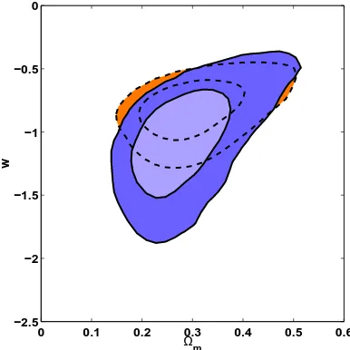
Figure 6.Marginalized 68% and 95% confidence contours from a combined analysis of the WMAP, ACBAR and CBI data together with a prior from BBN and HST, for an (incorrect) smooth dark energy component (dashed lines) and correctly including pertur-bations with ˆc2
s= 1 (solid lines).
provided by WMAP (Verde et al. 2003; Hinshaw et al. 2003; Kogut et al. 2003) (including the temperature-polarization cross-correlation data), we use CBI (Pearson et al. 2003) and ACBAR (Kuo et al. 2002) data for the smaller scales (ℓ >800).
per-w
log
10
(cs
2)
−2 −1.5 −1 −0.5 0
−3 −2 −1 0 1 2
Ωm
w
0 0.1 0.2 0.3 0.4 0.5 0.6 −2
−1.5 −1 −0.5 0
Figure 7.Marginalized 68% and 95% confidence contours from a combined analysis of the WMAP, ACBAR and CBI data together with a prior from BBN and HST, with ˆc2
s= 1 (dashed) and with ˆ
c2
svarying (solid).
turbations. This is a direct result of the difference between Figs. 2 and 3. Because the large ISW for w < −1 is not present if we include perturbations this part of the parame-ter space can not be excluded with CMB data. Furthermore the inclusion of perturbations leads to more stringent up-per bounds on the equation of state w. This is because as we increase the large scale CMB power due to the pertur-bations (for w > −1), the relatively low quadrupole and octopole disfavour these models. In Fig. 7 we show the con-straints from additionally varying a constant sound speed. This slightly favours values of w > −1, where low sound speeds lead to a smaller ISW contribution at the lowest ℓ. For w < −1 the contours broaden to include large sound speeds which also give somewhat smaller low multipoles.
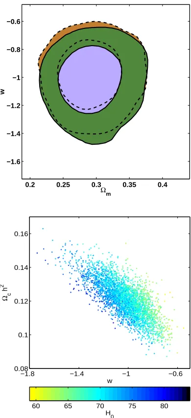
Finally we performed an analysis where we also in-cluded the data from the Supernovae Cosmology Project (SCP) (Perlmutter et al. 1999) and the two degree field (2dF) galaxy redshift survey (Percival et al. 2001). The in-formation from the 2dF large scale structure combined with the prior from the Hubble Key Project constrains the mat-ter contents, while the Supernovae (SNe) information is complementary. In Fig. 8 we show the result of this com-bined analysis, with and without marginalizing over a vary-ing sound speed ˆc2
s. The mean value for scalar field models with ˆc2
s = 1 is w =−1.02, strikingly close to a cosmologi-cal constant, however the 95% marginalized confidence limit −1.37 < w < −0.74 still allows a lot of room for differ-ent dark energy scenarios. Allowing for a differdiffer-ent value of the sound speed only slightly shifts the constraints onwto higher values, with the 95% result−1.32< w <−0.70. The dominant remaining degeneracies are illustrated in the scat-ter plot in Fig. 8, where we see how the constraints depend on the preferred value of the Hubble parameterH0.
Ωm
w
0.2 0.25 0.3 0.35 0.4
−1.6 −1.4 −1.2 −1 −0.8 −0.6
−1.8 −1.4 −1 −0.6
0.08 0.1 0.12 0.14 0.16
w Ωc
h
2
H
0
60 65 70 75 80
Figure 8.Top: 68% and 95% contours for a combined analysis of the CMB data, 2dF, SNe, HST and BBN with ˆc2
s = 1 (solid) and marginalizing over ˆc2
s (dashed). Bottom: Samples from the posterior distribution for ˆc2s= 1 with the same data as above.
4 CONCLUSIONS
In this note we have re-analysed the constraints on the equa-tion of state parameterwof dark energy mainly from CMB observations. We have emphasised the fact that it is essen-tial to include perturbations in the dark energy component to perform the analysis. The large scale anisotropies look very different when perturbations are included and it seems hard to use large scale CMB information to break the de-generacies.
non-canonical kinetic terms and a momentum cut-off might be a valid model for such a scenario (Armendariz-Picon et al. 2000; Carroll et al. 2003).
Finally we found as a posterior mean value for the equa-tion of state parameter w=−1.02, though this conclusion might depend somewhat on our choice of a constant equa-tion of state parameterisaequa-tion (Maor et al. 2002). Further-more we do not find significant constraints on the value of a constant speed of sound. We note that in a recent pa-per Bean & Dor´e (2003) find a 1−σ detection for a low sound speed. This is probably due to the fact that they keep parameters like the the physical matter density fixed. However cross-correlating the large scale CMB data with large scale structure measurements could improve these con-straints (Boughn & Crittenden 2003; Bean & Dor´e 2003).
To conclude a cosmological constant is certainly very consistent with the current data, however the 95% limits on the effective equation of state do not rule out most scalar field dark energy models. Hence we need better observations to constrain dark energy models and to be able to distin-guish them from a cosmological constant. While large scale CMB observations are limited by cosmic variance, the pro-posed Supernovae Acceleration Probe - SNAP could fulfil this objective (Weller & Albrecht 2002).
ACKNOWLEDGEMENT
We thank S. Bridle, A. Challinor, G. Efstathiou, W. Hu, M. Peloso, J. Ostriker, P. Steinhardt and D. Wands for use-ful discussions. In the final stages of this work we became aware that a similar analysis is performed by R. Bean and O. Dor´e and L. Boyle, A. Upadhye and P. Steinhardt, and we particularly thank O. Dor´e for useful discussions about that work. JW is supported by the Leverhulme Trust and a Kings College Trapnell Fellowship. The parallel computations were done at the UK National Cosmology Supercomputer Center funded by PPARC, HEFCE and Silicon Graphics / Cray Research. We further thank the Aspen Center of Physics, where this work was finalised, for their hospitality.
REFERENCES
Amendola L., 1999, Phys. Rev., D60, 043501
Armendariz-Picon C., Mukhanov V., Steinhardt P. J., 2000, Phys. Rev. Lett., 85, 4438
Bean R., Dor´e O., 2003, astro-ph/0307100
Boisseau, B., Esposito-Far`ese, G., Polarski, D., Starobin-sky, A. A., 2000, Phys. Rev. Lett., 85, 2236
Boughn S., Crittenden R., 2003, astro-ph/0305001 Burles S., Nollett K. M., Turner M. S., 2001, Astrophys.
J., 552, L1
Caldwell R., Dave R., Steinhardt P., 1998, Phys. Rev. Lett., 80, 1582
Carroll S. M., Hoffman M., Trodden M., 2003, astro-ph/0301273
Challinor A., Lasenby A., 1999, Astrophys. J., 513, 1 Coble K., Dodelson S., Friedman J., 1997, Phys. Rev. D,
D 55, 1851
Corasaniti, P. S., Bassett, B., Ungarelli, C., Copeland, E. J,, 2003, Phys. Rev. Lett., 90, 091303
DeDeo S., Caldwell R. R., Steinhardt P. J., 2003, Phys. Rev., D67, 103509
Ferreira P., Joyce M., 1998, Phys. Rev. D, D 58, 023503 Freedman W., et al., 2001, Ap. J., 553, 47
Hinshaw G., et al., 2003, Ap. J. S., 148, 135 Hu W., Sugiyama N., 1995, Astrophys. J., 444, 489 Kogut A., et al., 2003, Ap. J. S., 148, 161
Kosowsky A., Milosavljevic M., Jimenez R., 2002, Pys. Rev. D, 66, 063007
Kuo C. L., et al., 2002, astro-ph/0212289
Lewis A., Bridle S., 2002, Phys. Rev., D66, 103511 Lewis A., Challinor A., Lasenby A., 2000, Astrophys. J.,
538, 473
Maor I., Brustein R., McMahon J., Steinhardt P. J., 2002, Phys. Rev., D65, 123003
Melchiorri A., Mersini L., Odman C. J., Trodden M., 2002, astro-ph/0211522
Pearson T. J., et al., 2003, Ap. J., 591, 556 Peebles P., Ratra B., 1988, Ap. J., 325, L17 Percival W., et al., 2001, MNRAS, 327, 1297 Perlmutter S., et al., 1997, Ap. J., 483, 565 Perlmutter S., et al., 1999, Ap. J., 517, 565 Ratra B., Peebles P., 1988, Phys. Rev., D 37, 3406 Riess A., et al., 1998, Astron. J, 116, 1009
Riess A., et al., 2001, Ap. J., 560, 49 Sachs R., Wolfe A., 1967, Ap. J., 147, 735 Schuecker P., et al., 2003, A & A, 402, 53
Seljak U., Zaldarriaga M., 1996, Astrophys. J., 469, 437 Spergel D. N., et al., 2003, astro-ph/0302209
Verde L., et al., 2003, Ap. J. S., 148, 195