A Survey on Node Mobility Models on MANET Routing Protocols Page 854
A Survey on Node Mobility Models on MANET Routing Protocols
Ashish Gupta 1, Akhilesh Kosta 2, Akhilesh Yadav 3 Department of Computer Science and Engineering
Kanpur Institute of Technology, Kanpur
[email protected], [email protected], [email protected]
Abstract-A Mobile Ad-Hoc Network (MANET) is a self-configuring network of mobile nodes connected by wireless links to form an arbitrary topology without the use of existing infrastructure. Since MANETs are not currently deployed on a large scale, research in this area is mostly simulation based. Among other simulation parameters, the mobility model plays a very important role in determining the protocol performance in MANET. Thus, it is essential to study and analyze various mobility models and their effect on MANET protocols. In this paper, we study different mobility models proposed in the recent research literature and their performance of routing protocols Bellman Ford, Dynamic Source Routing (DSR) and Location Aided Routing (LAR1). In this study we have considered three mobility scenarios: Random Waypoint, Group Mobility and Freeway Models. These three Mobility Models are selected to represent possibility of practical application in future.
1. Introduction
In general, a Mobile Ad hoc NETwork (MANET) is a collection of wireless nodes communicating with each other in the absence of any infrastructure. Due to the availability of small and inexpensive wireless communicating devices, the MANET research field has attracted a lot of attention from academia and industry in the recent years. In the near future, MANETs could potentially be used in various applications such as mobile classrooms, battlefield communication and disaster relief applications.
To thoroughly and systematically study a new Mobile Ad hoc Network protocol, it is important to simulate this protocol and evaluate its protocol performance. Protocol simulation has several key parameters, including mobility model and communicating traffic pattern, among others. In this chapter and the next chapter we focus on the analysis and modeling of mobility models. We are also interested in studying the impact of mobility on the performance of MANET routing protocols. We present a survey of the status, limitations and research challenges of mobility modeling in this chapter.
The mobility model is designed to describe the movement pattern of mobile users, and how their location, velocity and acceleration change over time. Since mobility patterns may play a
significant role in determining the protocol performance, it is desirable for mobility models to emulate the movement pattern of targeted real life applications in a reasonable way. Otherwise, the observations made and the conclusions drawn from the simulation studies may be misleading. Thus, when evaluating MANET protocols, it is necessary to choose the proper underlying mobility model. For example, the nodes in Random Waypoint model behave quite differently as compared to nodes moving in groups [1]. It is not appropriate to evaluate the applications where nodes tend to move together using Random Waypoint model. Therefore, there is a real need for developing a deeper understanding of mobility models and their impact on protocol performance.
so-A Survey on Node Mobility Models on Mso-ANET Routing Protocols Page 855 called synthetic mobility models [2] that are not
trace-driven.
In the previous studies on mobility patterns in wireless cellular networks[3][4], researchers mainly focus on the movement of users relative to a particular area (i.e., a cell) at a macroscopic level, such as cell change rate, handover traffic and blocking probability. However, to model and analyze the mobility models in MANET, we are more interested in the movement of individual nodes at the microscopic-level, including node location and velocity relative to other nodes, because these factors directly determine when the links are formed and broken since communication is peer-to-peer.
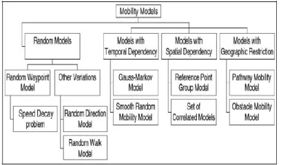
Figure 1. The categories of mobility models in
Mobile Ad hoc Network
In Fig.1 we provide a categorization for various mobility models into several classes based on their specific mobility characteristics. For some mobility models, the movement of a mobile node is likely to be affected by its movement history. We refer to this type of mobility model as mobility model with temporal dependency. In some mobility scenarios, the mobile nodes tend to travel in a correlated manner. We refer to such models as mobility models with spatial dependency. Another class is the mobility model with geographic restriction, where the movement of nodes is bounded by streets, freeways or obstacles.
2. Mobility Models
Different mobility models can be differentiated according to their spatial and temporal dependencies.
Spatial dependency: It is a measure of how two
nodes are dependent in their motion. If two nodes are moving in same direction then they have high spatial dependency.
Temporal dependency: It is a measure of how
current velocity (magnitude and direction) are related to previous velocity. Nodes having same velocity have high temporal dependency.
A. Random Waypoint
The Random Waypoint model is the most commonly used mobility model in research community. At every instant, a node randomly chooses a destination and moves towards it with a velocity chosen randomly from a uniform distribution [0,V_max], where V_max is the maximum allowable velocity for every mobile node. After reaching the destination, the node stops for a duration defined by the 'pause time' parameter. After this duration, it again chooses a random destination and repeats the whole process until the simulation ends. Figures 2-4 illustrate examples of a topography showing the movement of nodes for Random Mobility Model.
Figure 2. Topography showing the movement of
nodes for Random mobility model.
B. Random Point Group Mobility
A Survey on Node Mobility Models on MANET Routing Protocols Page 856 Random point group mobility can be used in
military battlefield communication. Here each group has a logical centre (group leader) that determines the group’s motion behavior. Initially each member of the group is uniformly distributed in the neighborhood of the group leader. Subsequently, at each instant, every node has speed and direction that is derived by randomly deviating from that of the group leader. Given below is example topography showing the movement of nodes for Random Point Group Mobility Model. The scenario contains sixteen nodes with Node 1 and Node 9 as group leaders.
Figure 3. Topography showing the movement of
nodes Random point group mobility
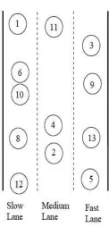
C. Freeway Mobility Model
This model emulates the motion behavior of mobile nodes on a freeway. It can be used in exchanging traffic status or tracking a vehicle on a freeway. Each mobile node is restricted to its lane on the freeway. The velocity of mobile node is temporally dependent on its previous velocity.
Figure 4. Topography showing the movement of
nodes for Freeway mobility model. Given below is example topography showing the movement of nodes for Freeway Mobility Model with twelve nodes.
3. Description of Routing Protocols
A. Bellman Ford Routing
Bellman-Ford Routing Algorithm, also known as Ford-Fulkerson Algorithm, is used as an algorithm by distance vector routing protocols such as RIP, BGP, ISO IDRP, and NOVELL IPX. Routers that use this algorithm will maintain the distance tables, which tell the distances and shortest path to sending packets to each node in the network. The information in the distance table is always updated by exchanging information with the neighboring nodes. The number of data in the table equals to that of all nodes in networks (excluded itself). The columns of table represent the directly attached neighbors whereas the rows represent all destinations in the network. Each data contains the path for sending packets to each destination in the network and distance/or time to transmit on that path. The Measurements in this algorithm are the number of hops, latency, the number of outgoing packets, etc.
B. Dynamic Source Routing (DSR)
A Survey on Node Mobility Models on MANET Routing Protocols Page 857 responses it receives. DSR allows the network
to be completely self-configuring without the need for any existing network infrastructure or administration. The DSR protocol is composed of two main mechanisms that work together to allow the discovery and maintenance of source routes in the ad hoc network. All aspects of protocol operate entirely on-demand allowing routing packet overhead of DSR to scale up automatically.
Route Discovery: When a source node S wishes to send a packet to the destination node D, it obtains a route to D. This is called Route Discovery. Route Discovery is used only when S attempts to send a packet to D and has no information on a route to D.
Route Maintenance: When there is a change in the network topology, the existing routes can no longer be used. In such a scenario, the source S can use an alternative route to the destination D, if it knows one, or invoke Route Discovery. This is called Route Maintenance [10] [11].
C..Location Aided Routing (LAR1)
Ad hoc on-demand distance vector routing (AODV) and distance vector routing (DSR) that have been previously described are both based on different variations of flooding. The goal of Location-Aided Routing (LAR) described in [6] is to reduce the routing overhead by the use of location information. Position information will be used by LAR for restricting the flooding to a certain area [7].
In the LAR routing technique, route request and route reply packets similar to DSR and AODV are being proposed. The implementation in the simulator follows the LAR1 algorithm similar to DSR.
Location Information When using LAR, any node needs to know its physical location. This can be achieved by using the Global Positioning System (GPS). Since the position information always includes a small error, GPS is currently not capable of determining a node’s exact
position. However, differential GPS5 offers accuracies within only a few meters.
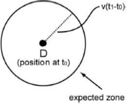
Expected Zone When a source node S wants to send a packet to some destination node D and needs to find a new route, it first tries to make a reasonable guess where D could be located. Suppose node S knows that at time t0 D’s position was P and that the current time is t1. Using this information S is able to determine the expected zone of D from the viewpoint of node S by time t1. For instance if D traveled with an average speed v, the source node S expects D to be in a circle around the old position P with a radius v(t1−t0). The expected zone is only an estimate by S to determine possible locations of D. If D traveled with a higher speed than S expected, the destination node may be outside the expected zone at time t1.
Figure 5. LAR Expected Zone
If the source node does not know the position of
D at time t0, it will not be possible to estimate an expected zone. D could be anywhere. In this case, the entire ad-hoc network is selected as the expected zone and the routing algorithm reduces to a simple flooding.
A Survey on Node Mobility Models on MANET Routing Protocols Page 858
• To create a path from S to D, both nodes must be contained in the request zone (Figure 6(a)). So if source S is not contained in the expected zone of D, additional regions need to be included. Otherwise the packet will not be forwarded from S to D.
• Under certain circumstances there may be no route from S to D, even if both nodes are contained in the requested zone (see Figure 6(b)). For instance, nodes that are near, but outside the request zone are needed to propagate the packet. Thus, after some timeout period, if no route is found from S to D, the request zone will be expanded and S will initiate a new route discovery process (Figure 6(c)). In this case, the route determination process will take longer because multiple route discoveries are needed.
C.1 LAR Request Zone Types
An intermediate node needs to use an algorithm to determine if it should forward a packet or not and if it is member of the request zone or not. LAR defines two different types of request zones in order to do this. LAR Scheme 1 (LAR1) was used in our simulations; it is discussed more detailed below. Further we mention LAR2 just for completeness.
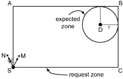
LAR Scheme 1 (LAR1) The request zone of LAR1 is a rectangular geographic region. Remember: If source node S knows a previous location P of destination node D at time t0, if it also knows its average speed v and the current time t1, then the expected zone at time t1 is a circle around P with radius r = v(t1 − t0). The request zone now is defined as the smallest possible rectangle that includes source node S
and the circular expected zone. Further should the sides of the rectangle be parallel to the x and
y axes.
Figure 6. LAR Scheme 1 - Request Zone
The source node is capable of determining the four corners of the rectangular request zone. This four coordinates are now included in the route request packet when initiating the route discovery process. Every node which is outside the rectangle specified by the four corners in the packet just drops the packet. As soon as the destination D receives the route request packet, it sends back a route reply packet as described in the flooding algorithms. Its reply differs by containing its current position, the actual time, and as an option its average speed. Source node
S is going to use this information for a route discovery in the future.
LAR Scheme 2 (LAR2) The second LAR scheme is defined by specifying (estimated) destination coordinates (xd, yd) plus the distance to the destination [7]. The estimated destination and the current distance to it are included in the route request. Now, a node may only forward the route request packet if it is closer or at maximum _ farther away than the previous node. _ is a system parameter which is dependent on implementation. Every forwarding node overwrites the distance field in the packet with its own current distance to the destination. This process ensures that the packet moves towards the destination.
4. Conclusion and Future Work
A Survey on Node Mobility Models on MANET Routing Protocols Page 859 hence the study results from one model cannot
be applied to other model. Hence we have to consider the mobility of an application while selecting a routing protocol.
Future study should be conducted to compare protocols in low mobility environment, where routes do not break to too often. Proactive protocols may give better performance for near stable environment. Performance of other routing protocol can be evaluated over various mobility models taking in to consideration number of average connected paths to gain greater insights into the relationship between them. Designing scenarios which depict real world applications more accurately can be designed through in-depth study of the application.
5. References
[1] S. Corson and J. Macker, Mobile Ad hoc Networking (MANET): Routing Protocol Performance Issues and Evaluation Considerations, RFC: 2501, January 1999.
[2] Carlo Kopp, “Ad Hoc Networking”, Systems Journal, pp 33-40,1999.
[3] Guolong Lin, Guevara Noubir and Rajmohan Rajaraman, "Mobility Models for Ad hoc Network Simulation", In Proceedings of IEEE INFOCOM 2004, Volume 1, pp. 7-11, 2004.
[4] Tracy Camp, Jeff Boleng and Vanessa Davies, “A Survey of Mobility Models for Ad Hoc Network” Special issue on Mobile Ad Hoc Networking: Research, Trends and Applications, vol. 2, no. 5, pp. 483-502, 2002.
[5] F. Bai and A. Helmy, "The IMPORTANT Framework for Analyzing and Modeling the Impact of Mobility in Wireless Adhoc Networks", in Wireless Ad Hoc and Sensor Networks, Kluwer Academic Publishers, 2004.
[6] F. Bai, A. Helmy, “A Survey of Mobility Modeling and Analysis in Wireless Adhoc Networks” in Wireless Ad Hoc and Sensor Networks, Kluwer Academic Publishers, 2004.
[7] F. Bai, G. Bhaskara and A. Helmy," Building the Blocks of Protocol Design and Analysis Challenges and Lessons Learned from Case Studies on Mobile Adhoc Routing and Micro-Mobility Protocols", ACM Computer Communication Review, Vol.34, No.3, pp.57-70, 2004.
[8] F. Bai, N. Sadagopan and A. Helmy, "IMPORTANT:A framework to systematically analyze the Impact of Mobility on Performance of Routing protocols for Adhoc Networks, IEEE INFOCOM, pp. 825-835, 2003.
[9] Charles E Perkins and Pravin Bhagwat, “Highly Dynamic Destination Sequenced Distance Vector Routing (DSDV) for Mobile Computers”, SIGCOMM 94, pp. 234-244, 1994.
[10] David B. Johnson, David A. Maltz, Yih-Chun Hu, The Dynamic Source Routing (DSR) Protocol for Mobile Ad Hoc Networks.draft-ietf-manet-dsr-10.txt, July 2004.
[11] David B. Johnson and David A. Maltz. “Dynamic Source Routing in Ad Hoc Wireless Networks”. In Mobile Computing, edited by Tomasz Imielinski and Hank Korth, Chapter 5, pages 153-181, Kluwer Academic Publishers, 1996.
[12] Biao Zhou, Kaixin Xu and Mario Gerla, “Group and Swarm Mobility Models for Ad Hoc Network Scenarios Using Virtual Tracks, In Proceedings of MILCOM’2004, Volume 1, pp. 289- 294, 1994.
[13] User Manual for IMPORTANT Mobility Tool Generator in NS-2 Simulator. Release Date February 2004.