DESIGN OF FEED FORWARD COMPENSATOR FOR A
THERMAL PROCESS
R.Ranjitha1, VijayRamrajRangam2, M.Suresh3
1PG student, EIE department, St. Joseph’s College of Engineering, Chennai - 600119 2
Assistant Professor,ICE department, St. Joseph’s College of Engineering, Chennai - 600119
3
Associate Professor, ICE department, St. Joseph’s College of Engineering, Chenna-119
Abstract: In this paper design of feedforward compensator for thermal process is proposed. The merits and demerits of feedforward and feedback control schemes are discussed. Feedforward compensators such as static, static with delay, Lead-Lag, and Lead-Lag designed and their performances are discussed in detailed using Matlab simulation. The effectiveness of feedforward controller also analysed with First order plus dead time (FOPDT) thermal process. Further nonlinearfeedforward controller also designed to improve disturbance rejection ability.
Keywords: Feed forward, FOPDT, PID controller,Compensator
I. Introduction
The PID controller treatment to both Steady state response and transient, most efficient solution to many real time process. The PID control schemes provide the advance in digital technology and science of automatic control in a wide spectrum. Feed forward controller is a system with a feed forward behavior which responds to the control signal in a predefined manner without taking into account the reaction of the load. Feed forward controller behaves contrary to feedback controller which adjusts the output by considering the reaction of the load. The feed forward control can be utilized for various applications such as drum level control. The design of feed forward compensator is very simple. An ideal feed forward compensator may have endless high frequency gain because of derivative exploit and its more difficult structure. Without any disturbance from the feedback controller the gain will be chosen the load is eliminated in steady state value [1].Different examples exists to illustrate the impact of disturbance on the controlled variable [2]. The disturbance that enters the control loop in the process is called as load disturbance. The main objective of this paper is to simultaneously improve local control performance and manage closed-loop coupling between pools by distributed control [3].The proportional term to providing the overall control action proportional to the error signal through all gain factor [4].
II. PROPOSED DESIGN OF FEEDFORWARD- FEEDBACK CONTROL
A. Basic relationships
A schematic diagram of feed forward – feedback control system is shown in Fig.1.
The Figure.1 consists of the basic feedback loop with feedback controller C, process P1 P2, and the signals
setpointysp , control signal u and process output y. A
measurable load disturbance d is influences the feedback loop according to the diagram, with transfer function P2 P3 between load d and process output y.
.
Fig.1: Block diagram of feedforward –feedback control
The disturbance effect on the output variable when the feed forward controller is implemented by the first order system with time delay alone may be written as 𝑃1 = 𝐾1 1+𝑆𝑇1𝑒 −𝑆𝐿1 ,𝑃 2= 𝐾2 1+𝑆𝑇2𝑒 −𝑆𝐿2 𝑃3= 𝐾3 1+𝑆𝑇3𝑒 −𝑆𝐿3 (1)
The transfer function of the PID controller is 𝐶 = 𝐾(1 + 1
𝑆𝑇𝑖+ 𝑆𝑇𝑎) (2)
The response of feedback control system Example 1:
For the simulation analysis, the process transfer functions are considered by assuming
K1 = K2 =1, K3 = 2, L1=L2 =1, L3 =2
The AMIGO tuning rules are:
PI CONTROLLER: 𝐾𝐶= 0.15 𝐾𝑝 + 0.35 − 𝐿 𝑇 (𝐿+𝑇)2 𝑇 𝐾𝑝𝐿 (3) 𝑇𝑖 = 0.35𝐿 + 13𝐿𝑇2 𝑇2+ 12𝐿𝑇 + 7𝐿2 PID CONTROLLER: 𝐾𝐶= 0.2 + 0.45 𝑇 𝐿 (4) 𝑇𝑖 = 0.4𝐿 + 0.8𝑇 𝐿 + 0.1𝑇 𝐿 𝑇𝑑 = 0.5𝐿𝑇 0.3𝐿 + 𝑇
The feedback controller parameters for Ziegler Nichols and AMIGO are shown in Table1
Table1 PID Controller parameters
Controller ZN AMIGO P Kp 0.96 PI Kp 0.872 0.25 KI 6.66 2.0 PID Kp 1.12 0.65 KI 4.0 1.09 KD 1.0 0.384
The servo and regulatory response of feedback controller is shown in figure 2 and 3.From servo and regulatory response, PID controller produced good response compared to other controllers. (i.e. P and PI controllers). The performance evaluation the based on ISE and IAE are analyzed and shown in Table 2 and Table 3.The working PID controller is analysed using ISE and IAE. The table shows PID controller produced good results compared to other controllers.
Figure2 Servo Response of feedback control system.
Figure 2 Regulatory response of feedback control system. Table.2 Error performance analysis of feedback control system
(Servo Response)
Controller ISE IAE
P 2706 52.02
PI 6.66 44.44
PID 3.96 15.99
Table 3 Error performance analysis of feedback control system (Regulatory Response)
Disturbance Controller ISE IAE
d=10% P 23.96 4.89 PI 0.66 0.44 PID 0.39 0.15 d=20% P 95.88 9.7 PI 1.33 1.77 PID 0.79 0.63 The comparison of servo and regulatory response of ZN and AMIGO tuning methods are shown in Figure 4(a) and 4(b).
Figure 4 Comparison of Servo response of feedback control system.
Figure 4(b) Comparison of regulatory response of feedback control system 0 10 20 30 40 50 60 70 80 90 100 0 0.2 0.4 0.6 0.8 1 1.2 1.4 Time (seconds) P r o c e s s v a r ia b le ) Setpoint P Controller PI Controller PID Controller 0 10 20 30 40 50 60 70 80 90 100 -0.02 0 0.02 0.04 0.06 0.08 0.1 0.12 0.14 Time (seconds) P r o c e s s V a r ia b le Setpoint P Controller PI Controller PID Controller 0 10 20 30 40 50 60 70 80 90 100 0 0.2 0.4 0.6 0.8 1 Time (seconds) P r o c e s s v a ia b le Setpoint PI-AMIGO PI-ZN 0 10 20 30 40 50 60 70 80 90 100 0 0.01 0.02 0.03 0.04 0.05 0.06 0.07 Time (seconds) P r o c e s s v a r i a b l e Reference PI-ZN PI-AMIGO
III. PERFORMANCE EVALUATION OF FEEDFORWARD CONTROL SYSTEM Proportional+ Integral+ Derivative (PID) controllers are mostly used in many industrial applications. The performance of the controller is heavily depends on the tuning parameters and less knowledge of the process alone sufficient to design them. The effective design of a controller is much easier nowadays due to the increase in computational capabilities. Feedback control does not provide predictive control action to recompense for the effects of known or assessableturbulence. The limitation of a PI controller is analyzed based on ISE, IAE on a conical tank level process. An auto tuning process controller with improved load disturbance rejection is presented. Traditional PID controllers cannot anticipate the disturbance inputs or the time evolution of the storage system.
A. Servo and regulatory response of feedforward control
Feedforward control is a controlling technique. The limitations of feedforward control are analyzed using simulation results.
Four structures of the feedforward compensator Gffare treated in this paper:
Static : 𝐺𝑓𝑓= 𝐾𝑓𝑓 (5)
Static with delay : 𝐺𝑓𝑓 = 𝐾𝑓𝑓𝑒−𝑆𝐿𝑓𝑓
Lead- Lag : 𝐺𝑓𝑓 = 𝐾𝑓𝑓
1+𝑠𝑇𝑍
1+𝑠𝑇𝑃
Lead-lag with delay :𝐺𝑓𝑓𝐾𝑓𝑓
1+𝑠𝑇𝑍
1+𝑠𝑇𝑃𝑒
−𝑆𝐿𝑓𝑓
More compound structures are seldom used in process control plants. In fact, the stable feedforward compensator is the most common structure, and feedforward by just a gain in the compensator can often make severe improvements in the control performance compared to pure feedback control.
B. Open-loop design
The open loop feedforward controller is intended by neglecting the feedback controller and also the effect of feedback on the troublenegative response. It means that the open-loop transfer function stuck between d and y is measured, which is given by
Y = P2(P3− P1Gff )D (6)
Perfect feedforward, which means that the effect of d is eliminated in y, is obtained when
𝐺𝑓𝑓= 𝑃3 𝑃1 = 𝐾3 𝐾1. 1+𝑠 𝑇1 1+𝑠 𝑇3𝑒 −𝑠(𝐿3−𝐿1) (7)
which means that
𝐾𝑓𝑓=
𝐾3
𝐾1, 𝑇𝑧= 𝑇1, 𝑇𝑃 = 𝑇3 ,
𝐿𝑓𝑓= 𝐿3− 𝐿1 (8)
when L3< L1, the optimal parameters given by (8), the feedforward compensator becomes negative. This means that ideal feedforward is not probable in this casing and feedforward compensator assumed to be Lff =0.
In this case a static feedforward controller
𝐺𝑓𝑓 = 𝐾𝑓𝑓 =
𝐾3
𝐾1 (9)
The feedforward compensator eliminates the effect of the disturbance in steady state.
A summary of the open-loop design rules designed for the different compensator Structures is:
Static : 𝐺𝑓𝑓=
𝐾3
𝐾1 (10)
Static with delay: 𝐺𝑓𝑓=
𝐾3 𝐾1𝑒 −𝑠(𝐿3−𝐿1) Lead –Lag : 𝐺𝑓𝑓= 𝐾3 𝐾1 1+𝑠𝑇1 1+𝑠𝑇3
Lead-Lag with delay : 𝐺𝑓𝑓= 𝐾3 𝐾1 1 + 𝑠𝑇1 1 + 𝑠𝑇3 𝑒−𝑠(𝐿3−𝐿1)
C. Design of feedforward compensator for L3 ≥ L1
The process transfer functions are 𝑃1 = 1 1+𝑠𝑒 −𝑠, (11) 𝑃2 = 1 1+𝑠𝑒 −𝑠, 𝑃3 = 1 1+2𝑠𝑒 −2𝑠
The feedback controller is PI controller tuned with AMIGO rule. The four different feedforward compensators are
Static : 𝐺𝑓𝑓= 1 (12)
Static with delay: 𝐺𝑓𝑓= 𝑒−𝑠
Lead –Lag : 𝐺𝑓𝑓=
1+𝑠 1+2𝑠
Lead-Lag with delay : 𝐺𝑓𝑓 =
1+𝑠
1+2𝑠𝑒
Figure 5.Response of feedforward compensator when L3≥L1
Figure 5 shows the load disturbance responses of four
different feedforward designs. The perfect feedforward is obtained when the lead-lag compensator with delay is used. When only static feedforward compensator is used large deviation in from the setpoint.
D. Design of feedforward compensator for L3< L1
The process transfer functions are 𝑃1 = 1 1+2𝑠𝑒 −2𝑠, (13) 𝑃2 = 1 1+𝑠𝑒 −𝑠, 𝑃3 = 1 1+𝑠𝑒 −𝑠
The PI controller is tuned with AMIGO rule. The four different feedforward compensators are
Static : 𝐺𝑓𝑓= 1 (14)
Static with delay :𝐺𝑓𝑓= 𝑒𝑠
Lead –Lag :𝐺𝑓𝑓=
1+2𝑠 1+𝑠
Lead-Lag with delay : 𝐺𝑓𝑓 =
1 + 2𝑠 1 + 𝑠 𝑒
𝑠
From Equation (14) the feedforward compensators static with delay and Lead-Lag with delay are physically unrealizable. In this case only static and Lead-Lag feedforward compensators are considered for the analysis. Figure 6 shows the response of feedforward controller when L3< L1. The static and
Lead-Lag compensators are not perfect compensators. Because of that there is deviation in the process output.
IV. DESIGN OF FEEDFORWARD COMPENSATOR FOR THERMAL
PROCESS
The performance of the feedback control depends mainly on the selection of suitable controller parameters, and the open loop transfer function of the
process. For many processes, it is very difficult to develop the fundamental mathematical process models to tune a specific control loop. However, it is possible to develop a transfer function based model by conducting a plant test. The well-known plant test is to give a step change in the manipulated input, and observe the measured process output. In this way, the best model has been developed, to provide an equal match between the model output and the practical plant output. The behaviour of the process is represented by a FOPDT model as
Ls PRC
e
1
s
K
)
s
(
G
(15)The process parameters are the static gain (K), the time constant (), and the dead time (L) of the plant derived from the transient response experiment using the step tuning method.
Consider, the FOPDT open loop transfer function of the process is s 12 p
e
1
s
34
1
.
1
)
s
(
G
(16)The disturbance process transfer function is
s 20 d
e
1
s
20
15
)
s
(
G
(17)Figure 6 Response of feedforward compensator when L3 < L1
A. Servo and Regulatory Responses of Feedforward-Feedback Controller
The limitations of feedforward control are analyzed using the simulation results. Using Equations (16) and (17) the transfer function of the feedforward controller is formulated as given in Equation (18). s 8 f
e
)
1
s
20
(
)
1
s
34
(
36
.
1
)
s
(
G
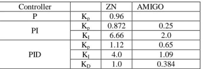
(18)The servo and regulatory responses of the feedforward – feedback control scheme is shown in Figure 7 0 50 100 150 -0.1 -0.08 -0.06 -0.04 -0.02 0 0.02 0.04 0.06 Time (seconds) P r o c e s s v a r ia b le Reference Static Lead-Lag Lead-Lag with dealy Static with delay
0 50 100 150 -0.15 -0.1 -0.05 0 0.05 0.1 Time (seconds) P r o c e s v a r i a b l e Reference Lead-Lag Static
Figure 7 Servo and regulatory responses of the FF-FBC The performance of the FF-FBC is analysed for different disturbance magnitudes (5%, 10%, 15% and 20%), for various modelling errors, such as process gain, time constant and combined process gain and time constant. The process gain is considered as 1.5 instead of 1.1. The servo and regulatory response, of the process with modelling errors is shown in Figure 8 (a - c) and its performance analysis is shown in Table 4. The deviation in the process variable due to modelling error, is very less compared to only the feedback control system. The designed FF-FBC is effective in eliminating the effects of the modelling errors. It is clear that the FFC is sensitive to modelling errors and the effects of modelling errors are eliminated by augmenting the FBC.
(a)
(b)
(c)
Figure 8 Servo and Regulatoryresponses of the FF-FBC with modelling errors at (a) 35% operating point, (b) 50% operating point and (c) 65% operating point
Table 4 Performance analysis of the FF-FBC with modeling errors Error
factors Disturbance
Servo and regulatory response of FF-FBC with modeling errors at various operating points
35% 50% 65%
ISE IAE ISE IAE ISE IAE
K=1.5 & τ =30 d=5% 330408.1 574.81 663503.3 814.55 1111817.6 1054.42 d=10% 348183.1 590.07 688548.3 829.78 1144229.3 1069.68 d=15% 366418.8 605.32 714103.0 845.04 1177101.8 1084.94 d=20% 385100.0 620.56 740438.6 860.48 1210695.4 1100.31 τ =30 d=5% 582206.2 763.02 1188174.4 1090.0 2008020.9 1417.04 d=10% 582203.9 763.02 1188174.1 1090.0 2008017.1 1417.04 d=15% 582201.9 763.02 1188173.6 1090.0 2008342.5 1427.16 d=20% 582294.0 763.02 1188160.5 1090.0 2007837.0 1416.98 K=1.5 d=5% 330408.0 574.81 663604.9 814.60 1111858.9 1054.44 d=10% 348183.0 590.07 688698.2 829.87 1144008.3 1069.58 d=15% 366423.9 605.32 714254.6 845.13 1176884.0 1084.84 . V. CONCLUSION
In this work, feedback and feedforward controller are designed and implemented. The merits and demerits of each controller scheme are discussed. An improved disturbance rejection is obtained using static, static with delay, Lead-Lag, Lead-Lag with delay feedforward compensators. Model uncertainties and disturbance effects are addressed, using the nonlinear feedforward controller. It improves the process output with the best rise time and less settling time, without design modifications.
In practice, most of the real time industrial stand data are linked with extent noise. The collection of sufficient, suitablegood qualityquality data is still a real problem.
REFERENCES
[1] Adam E. J ,Marchetti J. L. (2004). Designing and tuning robust feedforward controllers. Computers and Chemical Engineering 28 (2004) 1899–1911
[2] Guzmána J.L, Hägglund , T. (2011). Simple tuning rules for feedforward compensators. Journal of Process Control 21 (2011) 92–102.
[3] VladimírKučera(1998). Transfer function equivalence of feedback/feedforward compensator. kybernetika— volume 34 (1998), number 6, pages 610-624.
[4] Rossiter J.A. and Valencia-Palomowhich G. feedforward design in MPC.
[5] Ikuro Mizumoto1, Hiroki Tanaka1 and ZentaIwai2(2010). adaptive PID control for nonlinear systems with a parallel compensator. International Journal of Innovative Computing, Information and Control ICIC International c 2010 ISSN 1349-4198, Volume 6, Number 7, July 2010.
[6] Design and implementation of FPGA digital based PID controller(2014). Control Conference (ICCC), 2014 15th International Carpathian. May 2014
[7] Astrom, K, &Hagglund, T 2004, ‘Revisiting the Ziegler– Nichols step response method for PID control’, J. ProcessControl, vol. 14, pp. 635-650.
[8] Kaya, I 2004, ‘IMC based automatic tuning method for PID controllers in a Smith predictor configuration’, Computers and Chemical Engineering, vol. 28, pp. 281 – 290
[9] Padmashree, R, Srinivas, MN & Chidambaram, M 2004, ‘A simple method of tuning PID controllers for stable and unstable FOPTD systems', Computers and chemical engineering, vol. 28, pp. 2201- 2218. 0 500 1000 1500 0 10 20 30 40 50 60 70 Time (sec) P r oc e s s V a r ia bl e ( % ) Set Point Disturbance FFFBC 0 200 400 600 800 1000 1200 1400 1600 1800 2000 0 10 20 30 40 50 60 70 Time (sec) P roc e s s V a ri a bl e ( % ) Process gain Time Constant Process gain & Time Constant Disturbances (5% , 10% , 15% & 20%) 0 200 400 600 800 1000 1200 1400 1600 1800 2000 0 20 40 60 80 100 Time (seconds) P roc e s s V a ri a bl e ( % ) Process gain Time Constant Time constant & Process gain Disturbances (5%, 10%, 15% & 20%) 0 200 400 600 800 1000 1200 1400 1600 1800 2000 0 5 10 15 20 25 30 35 40 45 50 Time (sec) P roc e ss V a ri a bl e ( % ) Process gain Pocess gain & Time constant Time constant