Estimation of Population Ratio in Post Stratified Sampling Using Variable Transformation

http://dx.doi.org/10.4236/ojs.2015.51001

Estimation of Population Ratio in

Post-Stratified Sampling Using

Variable Transformation

Aloy Chijioke Onyeka, Chinyeaka Hostensia Izunobi, Iheanyi Sylvester Iwueze Department of Statistics, Federal University of Technology, Owerri, Nigeria

Email: [email protected], [email protected], [email protected]

Received 28 December 2014; accepted 16 January 2015; published 20 January 2015

Copyright © 2015 by authors and Scientific Research Publishing Inc.

This work is licensed under the Creative Commons Attribution International License (CC BY). http://creativecommons.org/licenses/by/4.0/

Abstract

Extending the work carried out by [1], this paper proposes six combined-type estimators of popu-lation ratio of two variables in post-stratified sampling scheme, using variable transformation.

Properties of the proposed estimators were obtained up to first order approximations,

( )

1

o n− ,

both for achieved sample configurations (conditional argument) and over repeated samples of fixed size n (unconditional argument). Efficiency conditions were obtained. Under these condi-tions the proposed combined-type estimators would perform better than the associated customa-ry combined-type estimator. Furthermore, optimum estimators among the proposed combined- type estimators were obtained both under the conditional and unconditional arguments. An em-pirical work confirmed the theoretical results.

Keywords

Variable Transformation, Combined-Type Estimator, Ratio, Product and Regression-Type Estimators, Mean Squared Error

1. Introduction

mean, ratio, proportion, etc.) under some realistic conditions, especially when there is a strong correlation be-tween the study variables and the auxiliary variables. Many authors have made contributions in this regard, in-cluding [2] and [3]. In this context, ratio, product and regression methods of estimation are good examples. Ra-tio and product-type estimators take advantage of the correlaRa-tion between the auxiliary variable and the study variable, to improve the estimate of the characteristic of interest. For example, when information is available on the auxiliary variable that is highly positively correlated with the study variable, the ratio method of estimation proposed by [4] is a suitable estimator to estimate the population mean, and when the correlation is negative, the product method of estimation, as envisaged by [5] and [6], is appropriate. However, in some studies, the ratio of the population means (or totals) of the study and auxiliary variables might be of great significance, hence the need to estimate such ratios.

The customary estimator of the population ratio

(

R=Y X

)

of the population means of two variables, y

and x, under the simple random sampling scheme, is given as Rˆ= y x, which is the ratio of the sample means of the two variables ([2] and [7]). The estimator, Rˆ= y x, uses information on only two variables, namely the study variable

( )

y and one auxiliary variable

( )

x . However, several authors, like [7] and [8], have contributed to the problem of estimating the population ratio of two means, often utilizing additional informa-tion on one or more auxiliary variables, say z i_i

(

=1, 2,

)

. While it is possible to record increased efficiency by introducing such additional auxiliary variables, it is obvious that extra cost is involved in order to obtain infor-mation on such additional auxiliary variables. References [1] and [9] have argued that such extra cost could be avoided by using variable transformation of the already observed auxiliary variable, instead of introducing addi-tional (new) auxiliary variables. However, the works carried out by [1] [9] were restricted to estimation of pop-ulation ratio in simple random sampling scheme. The present study is necessitated by the need to extend to post- stratified sampling scheme, the works on ratio estimation carried out by [1] [9] under the simple random sam-pling scheme. This is in order to extend to other samsam-pling schemes, the obvious advantage of reduced cost in the use of variable transformation instead of introducing additional (new) auxiliary variables when estimating pop-ulation ratio of two poppop-ulation parameters.

2. The Proposed Combined-Type Estimators

Let n units be drawn from a population of N units using simple random sampling method and let the sam-pled units be allocated to their respective strata, where nh is the number of units that fall into stratum h such

that

1

L

h h

n n

= =

∑

. Let yhi and xhi be the

th

i observation on the study and auxiliary variables, respectively. Consider the following variable transformation of the auxiliary variable, x, under post-stratified sampling scheme.

, 1, 2, , and 1, 2, ,

hi hi

NX nx

x h L i N

N n

∗ ₌ − _{= =}

−   (2.1)

An equivalent of the transformation (2.1), in simple random sampling scheme, has been used by authors like

[1] [8]-[13]. The associated sample mean estimator of the transformed variable (2.1), in post-stratified sampling scheme, can be written as

(

1

)

, where

ps ps

n

x X x

N n

π π π

∗ _{= − − =}

− (2.2)

and

1

L

ps h h

h

x ω x

=

=

∑

and

1

L

ps h h

h

y ω y

=

=

∑

are sample mean estimators based on xhi and yhi respectively. Using

the sample means yps, xps and xps

∗

, and assuming that the population mean, X of the auxiliary variable

hi

x , is known, we proposed six combined-type estimators of the population ratio R=Y X in post stratified sampling scheme as

(

)

1

ˆ ps

c

ps ps

y R

x b x∗ X

=

2

ˆ ps ps ps

c

ps ps

ps

y y x

R

x x X

X x ∗ ∗ = =         (2.4) 3

ˆ ps ps

c

ps ps

ps ps

y y X

R x x x x X ∗ ∗ = =       (2.5) 4 ˆ ps c ps y R x∗

= (2.6)

(

)

5 ˆ ps c ps ps y R

x∗ b x X

=

− − (2.7)

6

ˆ ps ps ps_.

c

ps ps

ps

y y x

R x X x X x ∗ ∗ = =         (2.8)

2.1. Conditional Properties of the Proposed Estimators

Reference [14] defined that under the conditional argument, that is, for the achieved sample configuration,

(

1, 2, 3, , L

)

n= n n n  n the post stratified estimator, yps is unbiased for the population mean, Y , with variance

( )

2

(

)

2 2 2 2

2

1 1 1

1 1

L L L

yh h yh

ps h h h yh

h h h h h

S S

V y f S

n n N

ω

ω ω

= = =

=

∑

− =

∑

−

∑

(2.9)

where V2 refers to conditional variance and 2

yh

S is the population variance of y in stratum h. Similarly, Onyeka (2012) obtained the conditional variance of xps and the conditional covariance of yps and xps

re-spectively as:

( )

2

(

)

2 2 2 2

2

1 1 1

1 1

L L L

xh h xh

ps h h h xh

h h h h h

S S

V x f S

n n N

ω

ω ω

= = =

=

∑

− =

∑

−

∑

(2.10)

and

(

)

2

(

)

2

2

1 1 1

1

, 1

L L L

yxh h yxh

ps ps h h h yxh

h h h h h

S S

C y x f S

n n N

ω

ω ω

= = =

=

∑

− =

∑

−

∑

(2.11)

where 2

xh

S is the population variance of x in stratum h, Syxh is the covariance of y and x in stratum

h, and C2 refers to conditional covariance.

Let

0 and 1 .

ps ps

y Y x X

e e

Y X

− −

= = (2.12)

Then, under the conditional argument,

( )

( )

2 0 2 1 0

E e =E e = (2.13)

( )

2 2

( )

2

(

)

2

2 0 2 2

1 1 1 L ps yh h h h h

V y S

E e f

n Y Y =ω

= =

∑

− (2.14)

( )

₂ 2

( )

₂

(

)

2

2 1 2 2

1 1 1 L ps _xh h h h h

V x _S

E e f

n X X =ω

( )

2

(

)

₂

(

)

2 0 1

1

, ₁

1 .

L

ps ps yxh

h h

h h

C y x S

E e e f

YX YX =ω n

= =

∑

− (2.16)

Using (2.12), the first proposed estimator, Rˆ1C, given in (2.3), can be re-written up to first order

approxima-tion, o n

( )

−1 , in expected value, as

(

)

(

)

(

)

(

)

2 2

1 0 1 0 1 1

ˆ _{1 1 1}

c

R −R =R e_ − +bπ e − +bπ e e + +bπ e _ (2.17)

and

(

)

(

)

2 ₂

2 2 2

1 0 1 0 1

ˆ _{1 2 1 .}

c

R R R e bπ e bπ e e 

 −  = + + − +

    (2.18)

We take conditional expectation of (2.17) and (2.18), and use (2.13) to (2.16) to make the necessary substitu-tions. This gives the conditional bias and mean square error of Rˆ1C respectively as

( )

(

)

2

(

)

2 1 2 22 12

1

ˆ _{1 1}

C

B R b RA b A

X π π

 

= _ + − + _ (2.19)

and

( )

(

)

2 2

(

)

2 1 2 11 22 12

1 ˆ

MSE RC A 1 b R A 2 1 b RA

X π π

 

= _ + + − + _ (2.20)

where

(

)

(

)

(

)

2 2 2 2 2

11 22 12

1 1 1

1 1 1

, , .

L L L

h h yh h h xh h h yxh

h h h h h h

f S f S f S

A A A

n n n

ω ω ω

= = =

− − −

=

∑

=

∑

=

∑

(2.21)

Following similar procedure, we obtain the conditional biases and mean square errors of the six proposed es-timators, together with those of the customary combined-type estimator, ˆRC = yps xps, of population ratio

( )

R , in post-stratified sampling, up to first order approximation, o n

( )

−1 , as:

( )

[

]

2 2 22 12

1 ˆ

C

B R RA A X

= − (2.22)

( )

(

) (

)

2 1 2 22 12

1

ˆ _{1 1}

C

B R b b RA A

X π π

= + _ + − _ (2.23)

( )

(

) (

)

2 2 2 22 12

1

ˆ _{1 1}

C

B R RA A

X π π

= + _ + − _ (2.24)

( )

(

2

)

(

)

2 3 2 22 12

1

ˆ _{1 1}

C

B R RA A

X π π π

 

= _ − + − − _ (2.25)

( )

2

2 4 2 22 12

1 ˆ

C

B R RA A

X π π 

= _ + _ (2.26)

( )

(

) (

)

2 5 2 22 12

1 ˆ

C

B R b b RA A

X π π

= + _ + + _ (2.27)

( )

(

)

[

]

2 6 2 22 12

1

ˆ ₁

C

B R RA A

X π π

= + + (2.28)

and

( )

2

2 2 11 22 12

1 ˆ

MSE RC A R A 2RA

X  

= _ + − _ (2.29)

( )

(

)

2 2

(

)

2 1 2 11 22 12

1 ˆ

MSE RC A 1 b R A 2 1 b RA

X π π

 

( )

(

)

2 2

(

)

2 2 2 11 22 12

1 ˆ

MSE RC A 1 R A 2 1 RA

X π π

 

= _ + + − + _ (2.31)

( )

(

)

2 2

(

)

2 3 2 11 22 12

1 ˆ

MSE Rc A 1 R A 2 1 RA

X π π

 

= _ + − − − _ (2.32)

( )

2 2

2 4 2 11 22 12

1 ˆ

MSE RC A R A 2 RA

X  π π 

= _ + + _ (2.33)

( )

(

)

2 2

(

)

2 5 2 11 22 12

1 ˆ

MSE RC A b R A 2 b RA

X π π

 

= _ + + + + _ (2.34)

( )

(

)

2 2

(

)

2 6 2 11 22 12

1 ˆ

MSE RC A 1 R A 2 1 RA .

X π π

 

= _ + + + + _ (2.35)

Generally, we have for the proposed six combined-type estimators,

( )

2 2

2 2 11 22 12

1 ˆ

MSE Rqc A qR A 2 qRA

X  θ θ 

= _ + − _ (2.36)

where q=1,, 6 and

(

)

(

)

(

)

(

)

(

)

1 1 b , 2 1 , 3 1 , 4 , 5 b , 6 1 .

θ = + π θ = +π θ = −π θ = −π θ = − π+ θ = − +π (2.37)

2.2. Unconditional Properties of the Proposed Estimators

Following [14] we obtain the following (unconditional) variances and covariance, for repeated samples of fixed size n.

( )

2

1

1 L

ps h yh

h

f

V y S

n =ω −

 

= _ _

∑

(2.38)

( )

2

1

1 L

ps h xh

h

f

V x S

n =ω −

 

=  

 

∑

(2.39)

and

(

)

1 1 Cov , L

ps ps h yxh

h

f

y x S

n =ω −

 

= _ _

∑

(2.40)

where f =n N is the population sampling fraction. By taking unconditional expectations of (2.17) and (2.18), and using (2.38)-(2.40) to make the necessary substitutions, we obtain the unconditional bias and mean square errors of the first proposed estimator, Rˆ_1c, up to first order approximation, o n

( )

−1 , as:

( )

1 2

(

)

(

)

22 12

1 1

ˆ _{1 1}

C

f

B R b b RA A

n

X π π

−

  _{′ ′}

= + _{  } + − _

  (2.41)

and

( )

(

)

2 2

(

)

2 2 11 22 12

1 1

ˆ

MSE C 1 2 1

f

R A R A RA

n

X π π

−

 _{  ′ ′ ′}

= _{  } + + − + _

  (2.42)

where

2 2

11 22 12

1 1 1

, , .

L L L

h yh h xh h yxh

h h h

A ω S A ω S A ω S

= = =

′ =

∑

′ =

∑

′ =

∑

(2.43)

Following similar procedure, we obtain the unconditional biases and mean square errors of the six proposed estimators, together with those of the customary combined-type estimator, ˆRC =yps xps, of population ratio

( )

R , in post-stratified sampling, up to first order approximation, o n

( )

−1 , as:

( )

2

[

22 12

]

1 1

ˆ

C

f

B R RA A

n X

−

  _{′ ′}

= _{ } −

( )

1 2

(

) (

)

22 12

1 1

ˆ _{1 1}

C

f

B R b b RA A

n

X π π

−

  _{′ ′}

= _{ } + _ + − _

  (2.45)

( )

2 2

(

) (

)

22 12

1 1

ˆ _{1 1}

C

f

B R RA A

n

X π π

−

  _{′ ′}

= _{ } + _ + − _

  (2.46)

( )

(

2

)

(

)

3 2 22 12

1 1

ˆ _{1 1}

C

f

B R RA A

n

X π π π

−

 _{  ′ ′}

= _{  } − + − − _

  (2.47)

( )

2

4 2 12 12

1 1

ˆ

C

f

B R R A A

n

X π π

−

 _{  ′ ′}

= _{  } + _

  (2.48)

( )

5 2

(

) (

)

22 12

1 1

ˆ

C

f

B R b b RA A

n

X π π

−

  _{′ ′}

= _{ } + _ + + _

  (2.49)

( )

6 2

(

)

[

22 12

]

1 1

ˆ ₁

C

f

B R RA A

n

X π π

−

  _{′ ′}

= _{ } + +

  (2.50)

and,

( )

2

11 22 12

2

1 1

ˆ

MSE R_C f A R A 2RA

n X

−

 _{  ′ ′ ′}

= _{  } + − _

  (2.51)

( )

2

(

)

1 2 11 22 12

1 1

ˆ

MSE R_C f A R 1 b A 2RA

n

X π

−

 _{  ′ ′ ′ }

= _{  } + + − _

  (2.52)

( )

(

)

2 2

(

)

2 2 11 22 12

1 1

ˆ

MSE C 1 2 1

f

R A R A RA

n

X π π

−

 _{  ′ ′ ′}

= _{  } + + − + _

  (2.53)

( )

(

)

2 2

(

)

3 2 11 22 12

1 1

ˆ

MSE R_C f A 1 R A 2 1 RA

n

X π π

−

 _{  ′ ′ ′ }

= _{  } + − − − _

  (2.54)

( )

2 2

4 2 11 22 12

1 1

ˆ

MSE R_C f A R A 2R A

n

X π π

−

 _{  ′ ′ ′ }

= _{  } + + _

  (2.55)

( )

(

)

2 2

(

)

5 2 11 22 12

1 1

ˆ

MSE R_C f A b R A 2 b RA

n

X π π

−

 _{  ′ ′ ′}

= _{  } + + + + _

  (2.56)

( )

(

)

2 2

(

)

6 2 11 22 12

1 1

ˆ

MSE R_C f A 1 R A 2 1 RA .

n

X π π

−

 _{  ′ ′ ′}

= _{  } + + + + _

  (2.57)

Generally, the unconditional mean square errors of the proposed combined-type estimators is obtained as

( )

2 2

11 22 12

2

1 1

ˆ

MSE R_qC f A _qR A 2 _qRA

n

X θ θ

−

 _{  ′ ′ ′ }

= _{  } + − _

  (2.58)

where θq, q=1,, 6 is as given in (2.37).

3. Efficiency Comparison

The efficiencies of the six proposed combined-type estimators are first compared with that of the customary combined ratio estimator RˆC in estimating the population ratio R of two population means under the

condi-tional and uncondicondi-tional arguments in post-stratified random sampling scheme. Secondly, the performances of the proposed estimators among themselves are investigated. Furthermore, the optimum estimators among the proposed estimators are also obtained. The efficiency comparison is carried out using the mean square errors of the estimators and the results are shown inTable 1.

4. Numerical Illustration

[image:7.595.85.539.195.314.2]

Statistics Department, Federal University of Technology Owerri to illustrate the properties of the estimators proposed in the present study. Absenteeism is measured as the average number of days absent from lectures in a month. The class consists of 50 students, with 32 and 18 students respectively falling into low-absenteeism (0 - 3 days per month) and high-absenteeism (4 - 6 days per month) groups or strata. Our interest is to estimate the ratio of final year GPA to absenteeism from lectures, based on a post-stratified sample of 20 out of the 50 gra-duating students in the class. The data statistics, consisting mainly of population parameters are shown inTable 2.

Table 3 shows the percentage relative efficiencies (PRE-1) of the proposed combined-type estimators, ˆRqc,

Table 1. Efficiency conditions under conditional and unconditional arguments.

Estimator Conditional argument Unconditional argument

qc

R is better than Rc if:

1) θ <q 1 and β<R

or

2) θ >q 1 and β>R

1) θ <q 1 and β′ <R

or

2) θ >q 1 and β′ >R

kc

R is better than Rjc if:

1) θj <θk and θj<β R

or

2) θj >θk and θj>β R

1) θj<θk and θj <β′ R

or

2) θj >θk and θj >β′R

qc

R is optimum if: 0

q R

θ =β 0

q R

θ =β′

[image:7.595.88.540.560.720.2]

Where β=A12 A22, β′=A12′ A22′ and θq, q=1,, 6 is as given in (2.37).

Table 2.Data statistics for final year GPA

( )

y and absenteeism from lectures

( )

x .

Population/sample parameters Stratum 1 (low-absenteeism) Stratum 2 (high-absenteeism)

50

N= N1=32 N2=18

20

n= n1=12 n2=8

(1−f)=0.60 (1−f1)=0.625 (1−f2)=0.556

2.98

Y= Y1=3.16 Y2=2.65

3.16

X= X1=2.03 X2=5.17

0.94

R= R1=1.56 R2=0.51

0.67

π= 2

1 0.2422

y

S = 2

2 0.0389

y S =

1 0.64

ω = 2

1 0.9990

x

S = 2

2 0.6176

x S =

1 0.2124

yx

S = − Syx2= −0.0161

1 0.64

ω = ω2=0.36

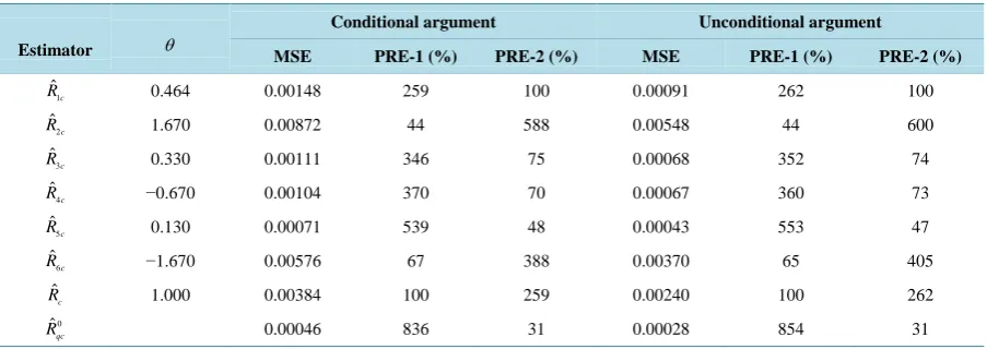
Table 3. Percentage relative efficiencies under conditional and unconditional arguments.

Estimator θ

Conditional argument Unconditional argument

MSE PRE-1 (%) PRE-2 (%) MSE PRE-1 (%) PRE-2 (%)

1 ˆ

c

R 0.464 0.00148 259 100 0.00091 262 100

2 ˆ

c

R 1.670 0.00872 44 588 0.00548 44 600

3 ˆ

c

R 0.330 0.00111 346 75 0.00068 352 74

4 ˆ

c

R −0.670 0.00104 370 70 0.00067 360 73

5 ˆ

c

R 0.130 0.00071 539 48 0.00043 553 47

6 ˆ

c

R −1.670 0.00576 67 388 0.00370 65 405

ˆ

c

R 1.000 0.00384 100 259 0.00240 100 262

0 ˆ

qc

over the customary combined-type estimator, ˆRc, under the conditional and under the unconditional arguments.

The table also shows the percentage relative efficiency (PRE-2) of the proposed combined-type estimators, Rˆ1c,

over the other combined-type estimators, under the conditional and under the unconditional arguments.

Table 3 shows that apart from the estimators, Rˆ2c and Rˆ6c, the remaining four proposed combined-type

es-timators, under the conditional and under the unconditional arguments, are more efficient than the customary combined-type estimator, Rˆc, for the data under consideration, and their gains in efficiency (PRE-1) are

rela-tively large. Also, using PRE-2, we observe that the proposed combined-type estimator, Rˆ1c, is more efficient

than the estimators, Rˆ2c, Rˆ6c, and Rˆc, under the conditional and unconditional arguments. The optimum

es-timator, as expected, has the highest gain in efficiency, both under the conditional and unconditional arguments. However, the customary combined-type estimator, on the other hand, is found to be more efficient than some of the proposed combined-type estimators for the given set of data. This confirms the theoretical results, which showed that the proposed estimators are not always more efficient than the customary combined-type estimator. Notice that β ′ = −0.16 and R=0.94 showing that β ′ <R and from the theoretical results inTable 1, the proposed estimators would be more efficient than the customary combined-type estimator, under the uncondi-tional argument, if θ_q <1. The empirical results inTable 3 show that θ2 >1 and θ6 >1, and the proposed

estimators Rˆ2 (PRE-1 = 44%) and Rˆ6 (PRE-1 = 65%) under the unconditional argument, are less efficient

than the customary combined-type estimator, Rˆc. Hence the empirical results confirm the theoretical results.

5. Concluding Remarks

The study extends use of variable transformation in estimating population ratio in simple random sampling scheme to post-stratified sampling scheme. Efficiency conditions for preferring the proposed estimators to the customary combined-type estimator are obtained. The study shows that in any given survey, these efficiency conditions should be employed in order to determine the appropriate proposed combined-type estimators to use for the purpose of estimating the population ratio of two variables in post-stratified sampling scheme, using va-riable transformation.

References

[1] Onyeka, A.C., Nlebedim, V.U. and Izunobi, C.H. (2013) Estimation of Population Ratio in Simple Random Sampling Using Variable Transformation. Global Journal of Science Frontier Research, 13, 57-65.

[2] Sukhatme, P.V. and Sukhatme, B.V. (1970) Sampling Theory of Surveys with Applications. Iowa State University Press, Ames.

[3] Cochran, W.G. (1977) Sampling Techniques. 3rd Edition, John Wiley & Sons, New York.

[4] Cochran, W.G. (1940) The Estimation of the Yields of the Cereal Experiments by Sampling for the Ratio of Grain to Total Produce. The Journal of Agricultural Science, 30, 262-275.

http://dx.doi.org/10.1017/S0021859600048012

[5] Robson, D.S. (1957) Application of Multivariate Polykays to the Theory of Unbiased Ratio-Type Estimation. Journal of the American Statistical Association, 52, 511-522.

http://dx.doi.org/10.1080/01621459.1957.10501407

[6] Murthy, M.N. (1964) Product Method of Estimation. Sankhya Series A, 26, 294-307.

[7] Singh, M.P. (1965) On the Estimation of Ratio and Product of the Population Parameters. Sankhya Series B, 27, 321- 328.

[8] Upadhyaya, L.N., Singh, G.N. and Singh, H.P. (2000) Use of Transformed Auxiliary Variable in the Estimation of Population Ratio in Sample Survey. Statistics in Transition, 4, 1019-1027.

[9] Onyeka, A.C., Nlebedim, V.U. and Izunobi, C.H. (2014) A Class of Estimators for Population Ratio in Simple Random Sampling Using Variable Transformation. Open Journal of Statistics, 4, 284-291.

http://dx.doi.org/10.4236/ojs.2014.44029

[10] Srivenkataramana, T. (1980) A Dual of Ratio Estimator in Sample Surveys. Biometrika, 67, 199-204.

http://dx.doi.org/10.1093/biomet/67.1.199

[11] Singh, H.P. and Tailor, R. (2005) Estimation of Finite Population Mean Using Known Correlation Coefficient between Auxiliary Characters. Statistica, 4, 407-418.

[13] Sharma, B. and Tailor, R. (2010) A New Ratio-Cum-Dual to Ratio Estimator of Finite Population Mean in Simple Random Sampling. Global Journal of Science Frontier Research, 10, 27-31.