Best First Heuristic Pruning Function for General Flow Shop Scheduling Problem

6

I

January 2018

Best-First Heuristic Pruning Function for General

Flow-Shop Scheduling Problem

Brahma Datta Shukla1 1

Ph.D. Scholar Swami Vivekanand University, Sagar (M.P.), India

Abstract: In this paper, primarily, best-first heuristic search with hill-climbing search implementation method has been expanded for general m-machine flow-shop scheduling problem, after that, a new pruning function of the branch and bound algorithm has been developed to control combinatorial explosion in the permutation schedule. This new pruning function tries to admit those partial schedule for advance extension and contemplation to get entire schedule, which give minimum amount of the idle times of all machines, and discards those partial schedules via which machines yield more than the minimum sum of the idle times. An illustration of numerical example is offered in sustaining of the best-first and new pruning function and algorithm. Performance of new heuristic pruning function has been assessed with overall lower bound.

Keywords: Make span, best-first search, heuristic pruning function, branch and bound etc.

I. INTRODUCTION

This is standard n-job and m-machine flow-shop (no-passing condition) scheduling problem by means of the objective function of reducing the time required to process all n jobs on all the m machines. This elapsed time is frequently known as make-span of a schedule.

Johnson, [1], one of the initiator, recommended a resolution that solves the case of two machines with optimality, recognized as the Johnson-rule. Here permutation sequences are prevailing, i.e. the job sequence is the equivalent for all machines. Additional optimization approaches comprises branch and bound [2], [3], elimination rules as in Baker [4], and row generation algorithms as in Frieze & Yadegar [5] and Dudek et al. [6]. Since the problems are ``NP-hard" where computational necessities for acquiring an optimal solution enhance exponentially as the problem size enhances [7], these techniques are computationally exhaustive for even very small size problems. Many methods have been build up to evade the computational complexity needed for attaining optimal solutions. Examples consist of transitive rules in Gupta [8], Woo and Yim [9], CDS algorithm in Campbell, Dudek, and Smith [10], priority rules in Mac Carthy and Liu [11], and the neighborhood outlawed search in Widmer and Hertz [12]. Though, there is no assurance if good schedules are produced.

James and Gupta[13] given a combinational procedure to resolve the restrained large flow-shop scheduling problems. Yadav and Chaudhari[14] executed their combinational procedure via linked list data structure to recover the problem size using Gupta’s[15] equation for adopting or discarding partial schedules. Ignall and Schrage[16] recommended branch and bound technique with lower bound pruning function for three-machine flow-shop sequencing problem.

This branch and bound technique has been extensive with best-first heuristic pruning function and minimum sum of idle time heuristic pruning function. Bansal, et. al [17] offered perception of global lower bound in which lower bounds are computed on job basis and also on machine basis which has been used as an benchmark to verify the optimality of the solution.

II. SCHEDULING CONDITIONS

Let X(i,j) indicate the time at which machine j initiates work on job i. And T(i,j) indicate the processing time of job i on machine j. Subsequently,

X(a,m) = Max [ X(a,m-1) + T(a,m-1) ; X(a-1,m) + T(a-1,m) ], …(1) Here , X(0,m) = X(a,0) = 0, for all a and m.

Formulation for the Terminal Point of the Algorithm

Partial Schedule: Any sequence of less than n jobs. Additionally, if the number of jobs is n then any sequence of n jobs is a complete schedule. For instance, if n = 4, then job sequences 2,4,3,1 and 3,1,4,2 are complete schedules where job sequences 1,2; 1,2,3; 2,1; 2,1,3; 4,1,3 etc. are partial schedules.

(1,3,4,2).In other terms, the sequence progresses to the right and is inferred as "followed by"; such as P followed by a. Let T(Pa,m) be the completion time of the partial schedule Pa on machine m. Taking into consideration equation (1) it is simple to expand a recursive relation for calculating T(Pa,m). We scrutinize that the m-th operation of the last job of the partial schedule P is on m-th machine, which processes the m-th operation of job a. Consequently, equation (1) simplifies as:

x(a,m) = Max [ T(Pa,m-1) ; T(P,m) ]

Since, T(Pa,m) = X(a,m) + T(a,m),

It follows that:

T(Pa,m) = Max [ T(Pa,m-1) ; T(P,m) ] + T(a,m); m

= 1,2,3,...m, …(2)

Where,

T(0,m) = T(Pa,0) = 0, for all Pa and m.

Now we can identify the m-machine flow shop scheduling problem as one of minimizing T(Pa,m), where P ranges above all possible permutations of n-1 jobs not containing job a, and job a ranges over all probable values from one through n. This explanation gives rise to n! possible schedules, each one of them being feasible. As of the factorial nature of the total number of feasible schedules, the problem still requires an appropriate method (efficient algorithm - polynomial order complexity) of searching an optimal schedule, excluding possibly for some particular cases.

III. IMPLEMENTING HEURISTIC SEARCH

The easiest mode to execute heuristic search is through a procedure called hill climbing due to Pearl, in George [18]. Hill-climbing strategies enlarge the current state in the search and assess its children. The best child is elected for extra extension; neither its siblings nor its parent are maintained. Search stops when it attains a state that is superior to any of its children. Here, in case of job scheduling, Search stops while all the jobs have been scheduled one by one. This approach of hill-climbing utilizes partial information; consequently probability of getting global optima is limited. Further informative algorithms similar to backtracking techniques with enhanced heuristic pruning function may be engaged for global optimal solution.

In spite of its restrictions, hill-climbing be capable of being used efficiently if the evaluation function is adequately informative to evade local maxima and infinite path. Generally, though, heuristic search entails a added flexible algorithm: this is provided by best-first search, where, with a priority queue, resurgence from local maxima is achievable. The comprehensive perceptions and formulation of job scheduling problem as heuristic search have been explained with an example problem. It is helpful to think of heuristic algorithms as consisting of two parts: the heuristic measure and an algorithm that uses it to explore the solution state space.

IV. BEST INTERIM MAKE-SPAN HEURISTIC MEASURE

If the intention of the scheduling problem is to reduce the completion time of all jobs on all machines, at that time it is expected to think of ways of scheduling or sequencing the jobs to reduce the make-span. So the creation of sequence or schedule ought to be such that the next job assigned to a machine be supposed to minimize the make-span. As a result, starting from the null partial

schedule and mainly escalating it by means of all unscheduled jobs one at a time, we get n partial schedules of each one job.

Calculate make-spans of all partial schedules. We can identify these make-spans as interim make-spans since these schedules are not

complete schedules of all n jobs. This interim make-span of a partial schedule might be a heuristic measure or criteria for deciding

which partial schedule can be extended to engender solution state space in the creation process of complete schedule in the heuristic search. Evidently, the partial schedule with minimum interim make-span may be established for further expansion and exploration. This is a simple standard to clarify the heuristic search method. This heuristic measure will work as a bound function which is

explained as: originally, create n partial schedules of one job each. Calculate their interim make spans for these partial schedules.

Determine a partial schedule Pi, such that, the interim make span of Pi (1  i  k, initially k = n) is minimum, then we discard or

prune all partial schedules other than Pi and accept Pi for additional expansion (branching) with unscheduled jobs, which are not in partial schedule Pi, to get complete schedule in the heuristic search, ultimately.

A. Algorithm

1) Step 1. Begin with null (which contains no job) partial schedule. Expand this null partial schedule by appending all unscheduled

jobs one by one. Thus, we get n partial schedules each including only one job.

3) Step 3. Evaluate the partial schedules with respect to their interim make-spans. Delete or reject those partial schedules that give up interim make-spans more than the minimum interim make-span (See illustration).

4) Step 4. Expand accepted partial schedule of step 3 by appending all unscheduled jobs for that partial schedule one by one.

5) Step 5.Recur step (2) through (4) until each partial schedule in step (4) contains n jobs i.e. complete schedule is attained.

6) Step 6. Calculate the make-spans of complete schedules of step (5). The minimum make-span schedules in step (5) are optimal or close to optimal solution.

B. Illustration

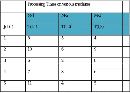
As an instance of the heuristic measure and algorithm just described, let us consider the five-job, three-machine flow shop scheduling problem of Table 1, below:

Processing Times on various machines

M-1 M-2 M-3

Job(I) T(I,1) T(I,2) T(I,3)

1 8 5 4

2 10 6 9

3 6 2 8

4 7 3 6

5 11 4 5

Table 1. A Five-Job, Three-Machine Scheduling Problem

We start with null partial schedule and augment it by all the five unscheduled jobs, thus, we get five partial schedules. Table 2 gives their completion times on all the three machines. The completion time on last i.e. on third machine is called as interim make-span. In table 2, the best i.e. the minimum interim make-span is 16 for partial schedules P3 = 3 and P4 =4.Therefore, as per the heuristic measure and algorithm, select both or any one or first one for convenience, for further expansion and prune or reject all other partial schedules.

Make-Span on Machines M-1 M-2 M-3

Partial

T(P,1)

T(P,2)

T(P,3)

Decision

Schedule(P)

1 8 13 17 Reject

2 10 16 25 Reject

3 6 8 16 Accept

4 7 10 16 Reject*

5 11 15 20 Reject

T(P, I) = Make-Span of Partial Schedule P on Machine I. T(P, 3) = Interim Make-Span of Partial Schedule P. * In case of tie select the first one.

Augment the accepted partial schedule P3 = 3 with all unscheduled jobs (1, 2, 4 and 5) one by one at a time. We get four partial schedules each of two jobs as shown in table 3. Interim Make-Spans of these Partial Schedules along with the decisions have also been shown.

Make-Span on Machines

Partial

T(P,1) T(P,2) T(P,3) Decision

Schedule(P)

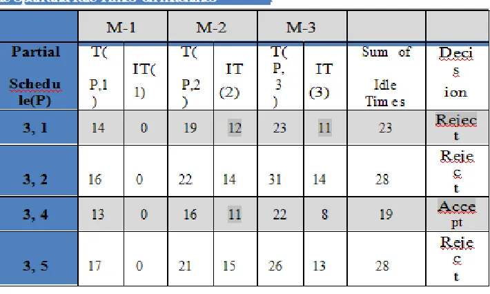
3, 1 14 19 23 Reject

3, 2 16 22 31 Reject

3, 4 13 16 22 Accept

3, 5 17 21 26 Reject

Table 3.Second list of Partial Schedules and their interim make-spans

Now we can evaluate the partial schedules of table 3 regarding their interim make-spans. In table 3, the best interim make-span is 22 for partial schedule P3 = (3, 4). As a result, we will admit partial schedule P3 for expansion with unscheduled jobs towards completion of this partial schedule and discard all other partial schedule as pointed to in the decision column of Table 3.

By progressing in this manner, we can complete the last column of Table 6. Because, the number of jobs in schedule of table 6 is 5

i.e. n, we get complete schedule and the make span of this schedule is 57 time unit, which might be optimal or near optimal one.

Make-Span on Machines

Partial

T(P,1) T(P,2) T(P,3) Decision

Schedule(P)

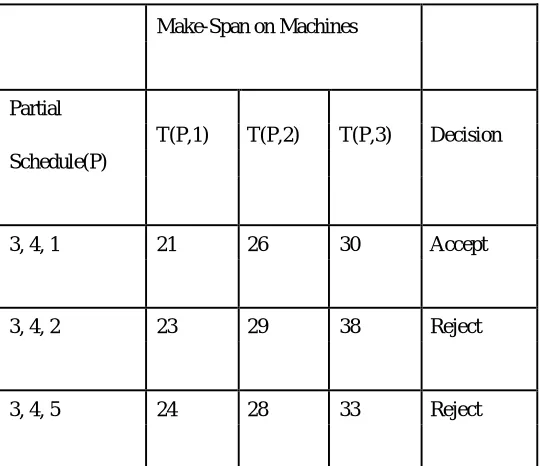
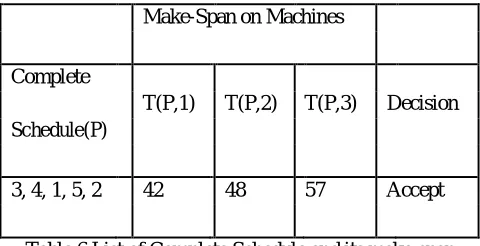
3, 4, 1 21 26 30 Accept

3, 4, 2 23 29 38 Reject

3, 4, 5 24 28 33 Reject

Make-Span on Machines

Partial

T(P,1) T(P,2) T(P,3) Decision

Schedule(P)

3, 4, 1, 2 31 37 46 Reject

3, 4, 1, 5 32 36 41 Accept

Table 5: Fourth list of Partial Schedules and their interim make-spans

Make-Span on Machines

Complete

T(P,1) T(P,2) T(P,3) Decision

Schedule(P)

3, 4, 1, 5, 2 42 48 57 Accept

Table 6.List of Complete Schedule and its make-span

One can’t be sure about the optimality of the solution obtained with heuristic methods unless until it has been checked with suitable yardstick. If the complete schedule of table 6 i.e. (3, 4, 1, 5, 2) is not optimal, after that further cautiously elected heuristic measure may yield improved solution as explained in the following section. Furthermore, the choices taken while breaking the ties may also influence the solution.

But, certainly, the search time gets condensed considerably, as, only one branch is explored at each iteration.

V. ANOTHER HEURISTIC MEASURE

Now, we solve the above similar problem by means of another heuristic measure i.e. minimum idle time on machines and evaluate the solutions attained by applying different heuristic functions and their effects.

A. Minimum Sum of Idle Time

If the goal is to reduce the total completion time of all jobs on all machines, at that time it is normal to think of ways of scheduling to decrease the idle times of machines. So the creation of sequence or schedule ought to be such that the next job allocated to a machine should minimize the idle phase of the machine. As a result, amount of the idle times of all machines for a partial schedule might be a heuristic measure or criteria for deciding which partial schedule can be extended to produce solution state space in the erection process of complete schedule in the heuristic search. Obviously, the partial schedule with minimum sum of idle times may be acknowledged for advance extension and exploration. This is one simpler heuristic criterion other than the traditional best-first search used in common heuristic search method. This heuristic measure will work as a bound function which is explained as:

primarily, generate n partial schedules of one job each. Calculate their make spans and sum of the idle times of all the machines for

these partial schedules. Decide a partial schedule Pi, such that, the sum of the whole idle times of Pi (1  i  k, initially k = n) is

B. Algorithm

1) Step 1. Begin with null (which contains no job) partial schedule. Expand this null partial schedule by appending all unscheduled

jobs one by one. Thus, we get n partial schedules each containing only one job.

2) Step 2. Compute their completion times (make-spans) and sum of total idle times on all machines.

3) step 3. Evaluate the partial schedules regarding their sum of total idle times. And delete or reject those partial schedules that provides sum of total idle times other than the minimum sum of total idle times (See illustration).

4) Step 4. Expand accepted partial schedules of step 3 by appending all unscheduled jobs for these partial schedules one by one.

5) Step 5.Recur step (2) through (4) until each partial schedule in step (4) contains n jobs i.e. complete schedule is attained.

6) Step 6. Calculate the make-spans of complete schedules of step (5). The minimum make-span schedule might be an optimal or near optimal solution.

C. Illustration

As an instance of this new heuristic measure and algorithm just explained, consider the same five-job, three-machine flow shop scheduling problem of Table 1.

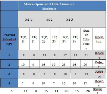
We begin with null partial schedule and expand it by all the five unscheduled jobs, accordingly we get five partial schedules. Table 7 provides their completion times, idle times on all the three machines and sum of overall idle times of all the machines. In table 7, the minimum sum of idle times is 14 for partial schedules P3 = 3. As a result, as per the heuristic measure and algorithm, choose this partial schedule for added extension and prune or discard all other partial schedules.

Table 7: First list of Partial Schedules and their sum of idle times

T(P, I) = Completion time of partial schedule P on machine I. IT(i) = Idle Time of machine i.

Make-Span and Idle Times on machines n

Machines

Table 8: Second list of Partial Schedules and their sum of idle times

In table 8, the minimum sum of idle times is 19 for partial schedule P3 = (3, 4). Consequently, we will admit partial schedule P3 for expansion with unscheduled jobs towards completion of this partial schedule and discard all other partial schedule as indicated in the decision column of Table 8.

By progressing in this mode, we will be capable of complete the last column of Table 11. as, the number of jobs in schedules of table 6 is 5 i.e. n, we got complete schedules and the minimum make span schedule is (3, 4, 1, 2, 5) with total completion time equal to 51 time unit, which might be optimal or near optimal one and acknowledged as our solution.

Make-Span and Idle Times onMachines

M-1 M-2 M-3

Sum

Partial T IT T IT T IT of

Decision

Schedu

(P,1 (1

(P,2 (2

(P,3 (3

Idle

le (P) )

) )

) )

)

Time

s

3, 4, 1 21 0 26 16 30 12 28 Accept

3, 4, 2 23 0 29 18 38 15 33 Reject

3, 4, 5 24 0 28 19 33 14 33 Reject

Make-Span and Idle Times on

Machines

M-1 M-2 M-3

Sum Partial T IT T IT T IT of

Decisi Schedu

(P,1 (1

(P,2 (2

(P,3 (3

Idle

on

le (P) ) ) )

) ) ) Time s

3, 4, 1,

31 0 37 21 46 19 40 Accept 2

3, 4, 1,

32 0 36

22 41 18 40 Accept 5

Table 10: Fourth list of Partial Schedules and their sum of idle times

Make-Span and Idle Times on

Machines

Sum

Partial T IT T IT T IT of

Decisi Schedu (P,1 (1 (P,2 (2 (P,3 (3 Idle on le (P) ) ) ) ) ) ) Time s

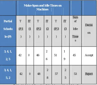
3, 4, 1,

42 0 46

2 51 1 45 Accept

2, 5 6 9

3, 4, 1, 42 0 48 2 57 2 53 Reject 5, 2 8 5

VI. CONCLUSION

While computing these results by means of the perception of global lower bound, we originate that the schedule (3, 4, 1, 2, 5) by means of entire completion time equal to 51 time unit is an optimal one, as the global lower bound value for this problem comes out to be 51. Consequently, we can conclude that the heuristic criterion the minimum sum of idle times of all machines not only discovers only one branch at most of the levels, but yields enhanced result or make span too. Therefore, we can observe that application of heuristic search on job scheduling optimization problem controls combinatorial explosion by pruning more branches at premature stages, which is enviable to save memory and reduce processing time.

REFERENCES

[1] Johnson, S., 1954: “Optimal two and three stage production schedules with setup times included”, Naval Research Logistics Quaterly, 1(1):61–68. [2] Lageweg, B.J., J. K. Lenstra, and A. H. G. Rinnooy Kan, 1978: “A General Bounding Scheme for the Permutation Flow-Shop Problem”, Operations

Research, Vol. 26, No. 1, January-February 1978, pp. 53-67.

[3] Richard L. Daniels, Joseph B. Mazzola, and Dailun Shi, 2004: “Flow Shop Scheduling with Partial Resource Flexibility”, Management Science, Vol. 50, No. 5, May 2004, pp. 658-669.

[4] Kenneth R. Baker, 1975: “A Comparative Study of Flow-Shop Algorithms”, Operations Research, Vol. 23, pp. 62-73.

[5] Frieze, A. M. and J. Yadegar, 1989: “A new integer programming formulation for the permutation flowshop problem”, European Journal of Operational Research, Vol. 40, pp. 90-98.

[6] Dudek, R.A., S.S. Panwalkar and M.L. Smith, 1992:“The lessons of Flowshop Scheduling Research”,Operations Research, Vol. 40, pp. 7-13.

[7] Teofilo Gonzalez, Sartaj Sahni, 1978: “Flowshop and Jobshop Schedules: Complexity and Approximation”, Operations Research, Vol. 26, No. 1, January-February 1978, pp. 36-52.

[8] Gupta, J.N.D., 1972: “Heuristic algorithms for multistage flowshop scheduling problem”, AIIE Transactions, 4, No. 1, pp. 11-18.

[9] Hoon-Shik Woo, and Dong-Soon Yim, 1998: “A heuristic algorithm for mean flow time objective in flow shop scheduling”, Computers and operations research Vol. 25, issue 3, pp. 175-182.

[10] Campbell, H.G., R.A. Dudek, and M.L. Smith, 1970: “A heuristic algorithm for the n job m machine sequencing problem”, Management Science, Vol. 16, No. 10, pp. 630-637.

[11] McCarthy B.L. and J. Liu, 1993: "Addressing the Gap inScheduling Research: A Review of Optimization and Heuristic Methods in Production Scheduling", International Journal of Prod. Research, Vol. 31, No. 1, pp. 59-79.

[12] Widmer, M., and A. Hertz, 1989: “A new Heuristic Method for the flow shop sequencing problem”,European Journal of Operational Research, Vol. 41 pp. 186-193.

[13] James, P.J. and Gupta, J.N.D. 1975: “Operations Research in Decision Making”, with the collaboration of Gerald R. Mc. Nichols, Crane Russak and Company, Inc. Newyork:292-296.

[14] Yadav, R.J. and Chaudhari, N.S. 2001: “Implementation of Optimal Schedule of Flow-shop Problem Using Linked-list Data Structure”, The Vikram Science Journal, Vikram University Ujjain, M.P. India.

[15] Gupta, J.N.D. 1972: “Optimal scheduling in a multi-stage flowshop.” AIIE Transactions 4:238-43.

[16] Ignall, E. and Schrage, L.E. 1965: “Application of theBranch and Bound Technique to Some Flow-Shopcheduling Problems”, Operations Research, XIII, No. 3, pp. 400-412.

[17] Bansal, S.P., Kalra, K.R. and Maggu, P.L. 1993:“Production Scheduling and Sequencing”, TechnocratPublications (March 1993).

ABOUT THE AUTHOR

Mr. Brahma Datta Shukla