Optimization of Grinding Process Parameters on CNC Grinding M/C using Taguchi Method

Optimization of Grinding Process Parameters on CNC Grinding M/C

using Taguchi Method

Mr. Akshay Bhole

Department of Production Engineering

Veermata Jijabai Technological Institute, Mumbai-400019, India

Abstract— In machining operations, one of the most

important machining processes is grinding process. It is responsible for producing discrete components with high precision which accounts for one fourth of the total expenditure of machining processes in industrialized nations. So it is very important for us to understood grinding process to improve surface finishing of products. Many researchers and investigators had proved that parameters such as work speed, wheel speed, depth of cut, feed rate, number of passes, etc are responsible for the effect on grinding process. Every parameter should have optimum value for better surface finish. Design of experiments is the best concept for optimization of parameters at the earliest stage of the processes. In this project, response variable selected is surface finish and input parameters selected are depth of cut, feed rate, work speed. Fractional factorial design is to be done by selecting orthogonal array for three factors and their three levels. Optimum grinding process parameters are to be selected using S/N ratios in Minitab software and ANOVA is to be done for identifying most dominating factor among all three parameters.

Keywords: Cylindrical Grinding, Surface Roughness, Orthogonal Array, Taguchi Method, Analysis of Variance, Plots

I. INTRODUCTION

Cylindrical grinding is the process of final finishing of components required for smooth surfaces and close tolerances. During the cylindrical grinding operations very

small size of the chips are produced. It is widely used in industry, grinding remains perhaps the least understood of all machining processes. In electric motor factory, motors are manufactured in which shaft is a component which should be precisely finished because it is mounted on bearings. Grinding should be done very precisely on the region of shafts where bearing is to be mounted and surface roughness should be minimum. The problem of mounting of bearings on shaft is due to variation in surface finish. The major operating input parameters that influence the output response of surface roughness are (i) Machine parameter (ii) Process parameter (iii) Grinding wheel parameter (iv) Work piece parameter[5]. There are noise parameters such as surrounding conditions, raw material variation, worker skill, etc which are uncontrollable. In this work i had taken work speed, feed rate, and depth of cut as process parameters that are influencing grinding process. Objective was to find out optimum levels of process parameters using taguchi method and most influencing parameter using analysis of variance. Also, analysis was done using main effect plot, interaction plot, contour plot.

II. EXPERIMENTAL DETAILS

A. Material Properties

In electric motors, material used for shaft was EN24 mild steel which is a popular grade of through-hardening alloy steel due to its excellent machinability in the "T" condition. EN24T is used in components such as gears, shafts, studs and bolts, its hardness is in the range 248/302 HB.

C Si Mn S P Cr Mo Ni

0.36- 0.10- 0.45- 0.040 0.035 1.00- 0.20- 1.30-

0.44% 0.35% 0.70% Max Max 1.40% 0.35% 1.70%

Table 1: Chemical composition of EN 24 steel

B. Measurement Tools

Measurement instrument used for measuring surface roughness of shaft was Mitutoyo SJ- 201 surface roughness tester profilometer which has a wide range from -200µm to +150µm. It is portable for easy measurement anywhere necessary and have large characters which are displayed on the large easy-to-view LCD.

C. Experimental Design

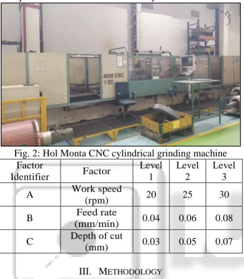
In this study, work speed, feed rate, depth of cut, wheel speed, number of passes were the main parameters which affects the surface roughness of material. Machine used for grinding on electric motor shafts was Hol Monta on which work speed was constant and we know that surface finish is directly proportional to number of passes. So that main three parameters selected were work speed, feed rate and depth of cut. The level of each grinding parameter was determined based on previous professional experience, brainstorming with professionals and literature survey.

Fig. 2: Hol Monta CNC cylindrical grinding machine Factor

Identifier Factor

Level 1

Level 2

Level 3

A Work speed

(rpm) 20 25 30

B Feed rate

(mm/min) 0.04 0.06 0.08

C Depth of cut

(mm) 0.03 0.05 0.07

III. METHODOLOGY

First of all the main functions and its side effects were identified, then all the factors that affects whole grinding process was identified i.e. controllable and uncontrollable (noise factors). Then identified the testing conditions like testing instrument, tool, workpiece material, etc and quality characteristics.

A. Orthogonal Array

Orthogonal array was selected after selecting factors and their levels. To select an ap- propriate orthogonal array, the total degrees of freedom needs to be computed. The degrees of freedom are defined as the number of comparisons between process parameters that need to be made to determine which level is better and specifically how much better it is[14]. Orthogonal array can be selected from minitab software as well as manually. So if values of parameters and levels was put in software, two orthogonal arrays i.e. L9 and L27 are shown. I had selected L9 orthogonal array for minimum number of experiments. Orthogonal array generated is below.

Experiment No. Control factors

A B C

1 1 1 1

2 1 2 2

3 1 3 3

4 2 1 2

5 2 2 3

6 2 3 1

7 3 1 3

8 3 2 1

9 3 3 2

Table 3: L9 Orthogonal Array

B. Conduction of experiment

A loss function is defined to calculate the deviation between the experimental value and the desired value. Taguchi recommends the use of the loss function to measure the performance characteristic First of all deviating from the desired value. The value of the loss function is further transformed into a signal-to-noise ratio (S/N)[14]. There are 3 Signal-to- Noise ratios of common interest which are called as objective function for optimization of Static problems.

Nominal the best, S/NT = -10 Log10 [ mean of sum of squares of measured data ]

Larger the better, S/NL = -10 Log10 [ mean of sum of squares of {measured - ideal}]

Smaller the better, S/NS = 10 Log10 (square of mean/variance)

Notice that, Nominal the best objective function is used when response value is a specified target, below or beyond which will not get optimized value. For ex, Aqua regia solution needs 1:3 of HNO3:HCL which is nominal value. Larger the better objective function is used when optimized response value is maximum for the system. Smaller the better objective function is used when optimized response value is minimum i.e zero for the system. Here smaller the better objective function for surface roughness should be taken to find out optimal machining performance. First of all 9 experiments were conducted according to selected orthogonal array and measured surface roughness values by surface roughness tester. Then S/N ratios were calculated using smaller the better performance characteristics. Scrap shaft (EN24 steel) of 2N-2735-41 series was taken for conducting the experiment which has diameter 130 mm and length 1521 mm. Speed of the wheel= 750 rpm, Width of the wheel= 110 mm, Spark out time= 3 sec, Time taken by wheel when no movement occurs before starting process= 6 sec.

Experime nt No.

Control factors

Measure d Surface Roughne

ss (Rz)

Calculat ed S/N Ratios (µm) Wor

k Spee

d (rpm

)

Feed rate (mm/mi

n)

Dept h of cut (mm )

1 20 0.04 0.03 2.12 -6.52672

2 20 0.06 0.05 2.98 -9.48433

3 20 0.08 0.07 3.63 -11.1981

4 25 0.04 0.05 2.46 -7.81870

5 25 0.06 0.07 2.16 -6.68908

6 25 0.08 0.03 2.76 -8.81818

7 30 0.04 0.07 2.02 -6.10703

8 30 0.06 0.03 2.00 -6.02060

9 30 0.08 0.05 2.32 -7.30976

IV. ANALYSIS

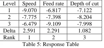
Main effect plots were generated from minitab software to find out optimum combinations of grinding process. The effect of a factor level is defined as the deviation it causes from the overall mean. For generating main effect plots, response table values should be calculated by taking average S/N ratio for same level experiments. Below is the response table for S/N ratios.

Level Speed Feed rate Depth of cut

1 -9.070 -6.817 -7.122

2 -7.775 -7.398 -8.204

3 -6.479 -9.109 -7.998

Delta 2.591 2.291 1.082

Rank 1 2 3

Table 5: Response Table

This values shows individual effects of factors and are commonly called as main effects. Rank in response table shows amount of influence factor affects on response variable. In above response table, rank is 1 for work speed it shows that work speed has more influence on surface roughness followed by feed rate and depth of cut.

The analysis of variance is done to investigate which of the following process parameters has more influence on response value. ANOVA table can be generated from minitab software or manually. This is accomplished by separating the total variability of the S/N ratios, which is measured by the sum of the squared deviations from the total mean of the S/N ratio, into contributions by each of the process parameters and the error[14]. First of all, overall mean of S/N ratios can be calculated as.

m = 1

9∑ (RZi

i=9

i=1 ) (1) where, m= overall mean of all S/N ratios, ηi = S/N ratio for ith _experiment.

The total sum of squared deviation is distributed in two sources i.e. sum of squared deviation for each process parameters SSP and sum of squared error SSe. Total sum of squared deviation & Sum of squares for each factor can be calculated by using effect of factors calculated in response table as:

Total sum of squares = ∑ (RZi− m)2 i=9

i=1 (2) Sum of squares due to factor A = [no. of experiments at level A1 * (mA1 - m)2] + [no. of experiments at level A2 * (mA2 - m)2] + [no. of experiments at level A3 * (mA3 - m)2] (3) Sum of squares due to factor B = [no. of experiments at level B1 * (mB1 - m)2] + [no. of experiments at level B2 * (mB2 - m)2] + [no. of experiments at level B3 * (mB3 - m)2] (4) Sum of squares due to factor C = [no. of experiments at level C1 * (mC1 - m)2] + [no. of experiments at level C2 * (mC2 - m)2] + [no. of experiments at level C3 * (mC3 - m)2] (5) where, mA1, mA2, mA3, mB1, mB2, mB3, mC1, mC2 & mC3 are the effect of factors A, B, C for level 1,2 & 3 resp.

The sum of squares for error is SSe = SST – (SSA + SSB + SSC) (6)

If t= no. of levels, n= no. of experiments, then total degree of freedom is DT = n-1 and degree of freedom for each testing parameter is DP = t-1. Mean squares are calculated as MSP = SSP /DP . Then, the F-value for each design parameter is simply the ratio of the mean of squares deviations to the mean of the squared error (MSP /MSe). Percentage contribution of factors can be calculated by taking percentage of sum of squared deviation for each factor with total sum of squares. F-test is performed to see which parameter has more influence on response variable. After calculating F-value, it is checked for larger and smaller for each factor because usually factor having larger F-value has more influence on performance characteristics.

V. RESULTS AND DISCUSSION

Effects of factors were calculated by taking average S/N ratios for same level experiments which was shown in table 5. Values in response table shows individual effects of factors and are commonly called as main effects.

A. Main Effect Plot

From the response table values main effect plots are plotted by taking all factors on X-axis and response table values on Y-axis.

Fig. 3: Main effect plot for S/N ratios

By taking values from response tables, main effects are plotted on single graph for S/N ratios. The goal in this experiment was to minimize the surface finish to improve the surface roughness of the LA8 series shafts produced through grinding process. Since –log depicts a monotonic decreasing function, we should maximize η or minimize surface roughness values Rz. Hence the optimum level for a factor is the level that gives the highest value of mean of η or lowest value of mean of Rz in the experimental region. Also after taking data means into considerations, optimum level is the level that gives the lowest value of surface roughness in experimental region. From figure 3 it is observed that the optimum settings of work speed, feed rate and depth of cut are A3, B1 and C1 if S/N ratios are taken into considerations. Hence results from main effect plot determines that the optimum grinding process parameters for minimum surface roughness are work speed= 30 rpm, feed rate= 0.04 mm/min and depth of cut= 0.03 mm.

Source DOF Adj SS Adj MS F-value P-value % contribution

Work Speed 2 10.067 5.0334 2.53 0.283 41.01

Feed rate 2 8.513 4.2566 2.14 0.319 34.68

Depth of cut 2 1.982 0.9910 0.50 0.668 8.07

Error 2 3.982 1.9909

Total 8 24.544

Table 6: Anova Table for S/N ratio Above Anova table was generated from minitab

software for S/N ratios and also checked for surface roughness mean values, but it can be calculated manually also. Data analysis for Taguchi method is done by ANOVA technique. Analysis indicates that percent of contribution by work speed is 41%, feed rate 34.5% and depth of cut 8% in both the conditions. This shows that work speed makes more influence on surface roughness and depth of cut has very low influence on roughness value. Also more the F-value greater will be the influence on surface roughness. So here work speed has more F-value in both conditions. Lesser the P-value more will be the influence on surface roughness. Here P-value is less for work speed in both conditions. Therefore, I can conclude that work speed is the most dominating factor & has more influence on surface roughness in grinding process.

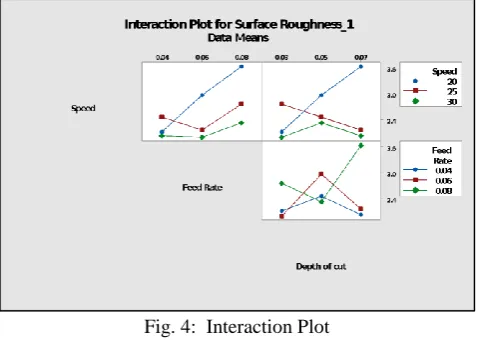
C. Interaction Plot

Interaction plots are used to show how the relationship between one categorial factor and a continuous response depends on the value of the second categorical factor. This plot displays means for the levels of one factor on the x-axis and a separate line for each level of another factor. So evaluate the lines to understand the effect of interaction on the relationship between the factors and the response. If there are parallel lines in plot, then no interaction occurs and if lines are nonparallel then interaction is present. The more nonparallel lines are, the greater the strength of the interaction. Here dependent variable is surface roughness and independent variables are work speed, feed rate, depth of cut. This interaction plot shows relationship between dependent variable and independent variable. Here in this interaction plot it seems that lines are not parallel.

Fig. 4: Interaction Plot

Now in first plot, it indicates that the relationship between work speed and surface roughness depends on feed rate. If we use speed 20 rpm then feed rate 0.04 mm/min is associated with lowest surface roughness and similarly if we use speed 25 rpm then feed rate 0.06 mm/min is associated with lowest surface roughness.

Second plot indicates that the relationship between speed and surface roughness depends on depth of cut. If we use speed 20 rpm then depth of cut 0.03 mm is associated with lowest surface roughness and if we use speed 25 rpm then depth of cut 0.07 mm is associated with lowest surface roughness value. Similarly third plot shows that relationship between feed rate and surface roughness depends on depth of cut. In these also different levels of factors are associated with different values of surface roughness. Therefore this Three-way ANOVA results indicate that the interaction between all these factors is significant.

D. Contour Plot

Fig. 4: Contour Plot

Use a contour plot to see how a response variable relates to two predictor variables. A contour plot provides a two dimensional view in which all points that have the same response are connected to produce contour lines of constant responses. Contour plots are useful for investigating desirable response values and operating conditions. This contour plot shows the relationship between work speed and feed rate used to improve the grinding process because depth of cut has no more influence on surface roughness so relationship of speed and feed rate affects the most. Minitab uses interpolation to create the area between data points. Dark region shows high surface roughness. In above plot lower right section is too much dark which shows very high surface roughness at high feed rate and lower work speed. Upper left section shows lowest surface roughness value at lower feed rate and higher speed. Also lower left section shows moderate surface roughness at lower feed rate and speed. Therefore best way is to use lower feed rate and higher work speed to get better surface finish on shafts of EN24 steel.

E. Confirmation test

surface roughness by conducting confirmation experiment. Theoretical value of surface roughness is calculated from regression equation formulated from Minitab software and practical value is measured by conducting confirmation experiment while considering optimum grinding process parameters. After getting optimum values of parameters, conduct the confirmation experiment same as conducted in above 9 experiments. Put the values of work speed as 30 rpm, feed rate as 0.04 mm/min, depth of cut as 0.03 mm in Siemens 840D panel and run the machine. Practical value of surface roughness after conducting experiment was 1.69 µm.

Regression equation formulated from minitab software is:-

Surface roughness = 2.494 + 0.416 Speed_20 – 0.034 Speed_25 – 0.381 Speed_30 – 0.294 Feed Rate_0.04 – 0.114 Feed Rate_0.06 + 0.409 Feed Rate_0.08 –0.201 Depth of cut_0.03 + 0.092 Depth of cut_0.05 + 0.109 Depth of cut_0.07.

For calculating theoretical value consider those values from the above equation which are variables of optimum parameters.

Therefore,

Surface roughness = 2.494 - 0.381 - 0.294 - 0.201 Surface roughness = 1.618 µm

Deviation = Practical value – theoretical value Deviation = 1.69-1.618 = 0.072 µm

Deviation between theoretical and practical value is the error caused due to human, process, machine, etc. So, the surface roughness value is optimized from 2.49 µm to 1.69 µm.

VI. CONCLUSION

 First of all response table values are calculated through S/N ratios. From these values main effect plots are plotted. By studying main effect plots i conclude that the optimum combinations of grinding process parameters for surface roughness using Taguchi design of experiment methodology are work speed: 30 rpm, feed rate: 0.04 mm/min, depth of cut: 0.03 mm.  Analysis of variance is done from which i can

conclude that percentage contribution of work speed on response is 41%, feed rate is 34.5% and depth of cut is 8%.

 In Anova table F-value of work speed is more for both data means and S/N ratios. Also p-value generated from software is lowest for work speed.

 Above discussion conclude that work speed has more influence on surface roughness out of three grinding parameters for EN24 steel material of LA8 series motor. Work speed is most dominating factor followed by feed rate which has lower influence and depth of cut has very weak influence on surface roughness.  Confirmation experiment is conducted after finding

optimum values from main effect plots and it shows that surface roughness value is optimized from 2.49 to 1.69 µm.

REFERENCES

[1] D. D. Mohite, S. M. Jadhav, An Investigation of Effect of Dressing Parameters for Minimum Surface Roughness using CNC Cylindrical Grinding Machine, International Journal of Research in Engineering and Applied Sciences VOLUME 6 (6).

[2] F. HOLESOVSKY, B. PAN, M. N. MORGAN, Andrej CZAN, Evaluation of Diamond Dressing Effect on Workpiece Surface Roughness by Way of Analysis of Variance, Tehničkivjesnik 25 (1) (0) 165–169.

[3] V. K. . M. M. Jagadeesh, Optimization of Cylindrical Grinding Process Parameters of OHNS Steel (AISI 0-1) Rounds Using Design of Experiments Concept, International Journal of Engineering Trends and Technology (IJETT) – Volume 17 Number 3 (2014) 109. [4] K. P. . N. Alagumurthi, V. Soundararajan, Optimization of Grinding Process Through Design of Experiment (DOE)—A Comparative Study, Vol. 21, 2006.

[5] S. K. . N. K. M. Ganesan, Prediction and Optimization of Cylindrical Grinding Parameters for Surface Roughness Using Taguchi Method, IOSR Journal of Mechanical and Civil Engineering (IOSR-JMCE) e-ISSN: 2278-1684.

[6] Srinivas Athreya, Dr Y.D.Venkatesh, Application Of Taguchi Method For Optimization Of Process Parameters In Improving The Surface Roughness Of Lathe Facing Operation, in: International Refereed Journal of Engineering and Science (IRJES) ISSN (Online) 2319-183X, Vol. 2319, 2012, pp. 13–19.

[7] Xun Chen & Tahsin T. Opoz, Effect of different parameters on grinding efficiency and its monitoring by acoustic emission, Production &Manufacturing Research An Open Access Journal ISSN, ISSN: (Print, pp. 2169– 3277.

[8] D. Patil, P. G. Chougule, M. A. Morale, S. D, Salunkhe, Review of Failure of Grinder Wheel.

[9] M. K. Sinha, D. Setti, P. V. R. Sudarsan Ghosh, An investigation into selection of optimum dressing parameters based on grinding wheel grit size, in: 5th International & 26th All India Manufacturing Technology, Design and Research Conference.

[10]R. Bauer, Abdalslam Darafon, Characterization of grinding wheel topography using a white chromatic sensor, International Journal of Machine Tools & Manufacture 70 (2013) 22–31.

[11]Ostertagova, Oskar Ostertag, Methodology and Application of One-way ANOVA, American Journal of Mechanical Engineering 2013 (1) 256–261.

[12]R. B. . D. Doman, A survey of recent grinding wheel topography models, International Journal of Machine Tools & Manufacture 46 (2006) 343–352.

[13]G. S. . M. Nalbant, Application of Taguchi method in the optimization of cutting parameters for surface roughness, Vol. 28.

[15]M. . Krishankant, Rajesh Kumar, Application of Taguchi Method for Optimizing Turning Process by the effects of Machining Parameters, Issue-1, 2012.

[16]P. B. S. Patel, P. R. G. Jivani, Design Of Experiments And Response Surface Method, in: Context To Grinding Process, National Conference on Recent Trends in Engineering &, Technology.

[17]S. A. Umredkar, Yash Parikh, Application of Taguchi method in optimization of control parameters of grinding process for cycle time reduction, in: International Journal of Innovative Research in Advanced Engineering (IJIRAE) ISSN: 2349-2163 Issue, Vol. 2, 2015, pp. 220– 229.

[18]Arshad Noor Siddiquee, Zahid A. Khana, Pankul Goel, Mukesh Kumar, Gaurav Agarwal, Noor Zaman Khan, Optimization of Deep Drilling Process Parameters of AISI 321 Steel using Taguchi Method, 2014.

[19]Prashant J. Patil, C.R. Patil, Analysis of process parameters in surface grinding using single objective Taguchi and multi-objective grey relational grade, Perspectives in Science (2016) 8, 367-369.

[20]Zhao Tao, Shi Yaoyao, Sampsa Laakso, Zhou Jinming, Investigation of the effect of grinding parameters on surface quality in grinding of TC4 titanium alloy, Procedia Manufacturing 11 ( 2017 ) 2131 – 2138. [21]S.A. Kryukov, A.S. Kryukov, Determining the

Parameters of Grinding Wheels Working Surface Profile, International Conference on Industrial Engineering, ICIE 2017, Procedia Engineering 206 (2017) 204–209.

[22]Arshad Noor Siddiquee, Zahid A. Khan, Pankul Goel, Mukesh Kumar, Gaurav Agarwal, Noor Zaman Khan, Optimization of Deep Drilling Process Parameters of AISI 321 Steel using Taguchi Method, Procedia Materials Science 6 ( 2014 ) 1217 – 1225.