Closed loop control using a backpropagation algorithm: a practicable approach for energy loss minimisation in electrical drives

item and our policy information available from the repository home page for further information.

Author(s):Matieni, Xavier; Dodds, Stephen J.; Lee, Sin W.

Title:Closed-loop control using a backpropagation algorithm: a practicable approach for energy loss minimisation in electrical drives.

Year of publication:2010

CLOSED-LOOP CONTROL USING A BACKPROPAGATION

ALGORITHM: A PRACTICABLE APPROACH FOR ENERGY

LOSS MINIMISATION IN ELECTRICAL DRIVES

Xavier Matieni, Stephen J. Dodds and Sin W. Lee

School of Computing, Information Technology and Engineering, University of East London [email protected], [email protected], [email protected]

Abstract: In general, optimal controls are computed off line and subsequently applied in real time but this approach is impracticable due to lack of robustness with respect to the plant modelling errors and unknown external disturbances. Closed loop versions of these optimal controls could circumvent this problem but are only available in the analytical form for very simple cases, not including minimisation of frictional energy loss in motion control systems, which is the aim of the research programme. The approach suggested by Matieni and Dodds (2009), however, overcomes this obstacle by training an artificial neural network (ANN) to reproduce the optimal control values computed off-line from given states and reference inputs, thereby yielding a closed loop solution. The purpose of this paper is to present the results of an initial simulation experiment to assess the capability of a Multilayered Perceptron (MLP), in the backpropagation mode, to perform a direct state feedback function, which, to the authors‘ knowledge, is new. A known linear state feedback controller for a double integrator plant is used for this purpose. The control law is used to train the MLP. Then a simulation of the closed loop system formed using this MLP is compared with a simulation of the known linear state feedback control system. The results show that the closed loop step response with the MLP closely follows that of the conventional system.

1. Introduction

The long established open loop methods of Bellman et. al. (1962), known as ‗Dynamic Programming‘, in the USA and Pontryagin (1960), a Russian mathematician, with the ‗Maximum Principle‘, compute optimal

controls off line and apply them

subsequently in real time. During the period

leading up to the 21st century, these methods

have been abandoned by the mainstream control researchers due to the fundamental

drawback of susceptibility to plant

modelling errors and external disturbances and the lack of success in overcoming this drawback by deriving closed loop versions in all but the simplest and often unrealistic cases.

Bryson et. al. (1975) in his works on the

numerical solution of optimal programming

and control problems, investigated the possibility of closing the loop iteratively by the gradient method. The first-order gradient

and second-order gradient methods

demonstrated vast improvements in the first iterations but, unfortunately, displayed poor overall convergence, which means that the optimal solution could not be obtained fast enough for real time implementation. Also Ryan (1982) stated that explicit optimal closed-loop solutions have been obtained in a variety of cases of up to fourth order but

frequently exhibit a high level of

complexity, which may prove to be unacceptable in many practical applications. This is especially evident in the time-optimal feedback control laws for certain third and fourth-order plants, many of which

involved logarithmic and exponential

computationally too demanding for commonly used digital processors in many

control applications. He carried out

investigations of third and fourth-order linear, single-input plants, and nonlinear, multi-input plants some of which exhibited such complexity that explicit closed-loop solutions are not available at the present and unlikely to be obtained in the future. The method pursued in this research programme circumvents these difficulties.

In principle, an MLP can mimic any

continuous state feedback controller

yielding smooth outputs. During the training process, the parameters of the network, i.e., the neuron input weights, are being adjusted to minimise the error between the desired control input, u, and the control input, unn, generated by the neural network. The ultimate aim is to use the MLP to reproduce the function of the computed optimal controls referred to above but in a closed loop control structure with the possibility of yielding some robustness against plant modelling errors and external disturbances, as proposed by Matieni and Dodds (2009). This paper, however, is restricted to a first step in which the ability of an MLP to reproduce the behaviour of a simple linear state feedback control law for a double integrator plant is investigated.

The conventional performance measure for MLP training is the mean-square error or the sum of the squared errors over the training sample. Such a performance measure is a function of the free parameters of the system, i.e., the neuron input weights. This

function may be visualized as a

multidimensional error-performance surface with the free parameters as coordinates. It is important to note here that the MLP has really provided an approximation to a function of several variables. In the single input plant control application, it is the

control variable as a function of the plant state variables and the reference input.

2. Simulation of the MLP realisation

of linear state feedback control of a

double plant:

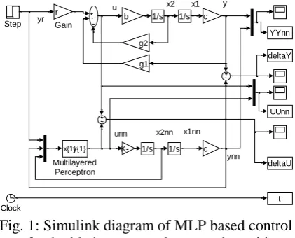
A linear second order plant model is accurate enough for many real applications found in the fields of spacecraft control; chemical process control, bio-engineering, aircraft control, etc. This justifies the use of a double integrator plant for this initial investigation. Fig. 1 shows the Simulink block diagram of the conventional linear state feedback control, used as a standard of comparison for the trained MLP controller.

yr u x2 x1nn unn y x2nn ynn x1 1/s 1/s deltaU UUnn YYnn deltaY t Step x{1}y{1} Multilayered Perceptron c c r Gain 1/s 1/s Clock g1 g2 -K-b

Fig. 1: Simulink diagram of MLP based control of a double integrator plant together with

conventional control as bench mark.

The plant states, x1 and x2 are available to the

conventional linear state feedback control law and the plant states, x1nn and x2nn, are

available to the MLP based control law, together with the reference input yr. Applying

Mason‘s rule to derive the desired closed loop transfer function for the conventional system yields

2

2 1

r

y s rbc

y s s bg s bg . (1)

unity DC gain and a settling time (5% criterion) using the 5% settling time formula of Dodds (2008) with n= 2:

n 2

1.5 1 4.5 9 2

s c c c

T n T T T (2)

where T_c is the time constant of the identical first order cascaded subsystems of which the required closed loop system can be considered to be composed. Hence the desired closed loop transfer function is:

2 2 2 s 2 2 s 9 2 1

s 1 s 9 2

81

4 s

4

s 9 81

s c

r c s

s

y s T T

y s T T

T

T T

(3) Comparing (1) and (3) then yields the controller gains

1 2 2

81 9

,

4 _{s s}

g g

bT bT

(4) and the reference input scaling coefficient

2 81

4 _s

r

bcT

The closed loop control law is then

1 1 2 2

r

u ry g x g x

(5) With the same plant states x1, x2 and the

reference input, yr, the MLP controller will

be trained to reproduce an input variable,

unn, of the same value as u from the

conventional controller, using (5).

The m-file used for the MLP training is as follows:

M-file

%%Position control c=5

b=3

%%Demanded settling time [s] Ts=0.2

g1=81/(4*b*Ts^2*c) g2=9/(b*Ts)

r=81/(4*b*Ts^2*c)

yr=[1 -1 1 -1 1 -1 1 -1 1 -1 1 -1 1 -1 1 -1 1 -1 1 1 1 0 0 -1 0 1 -1 -1 1 0 -1 -2 2 -2 2 1 2 1 1 -1 0 2 -2 2 2 -1 2 3 -3]

x1=[0 0 .0455 .0455 .1074 .1074 .1503 .1503 .1749 .1749 .1878 .1878 .1942 -.1942 .2 -.2 0 0 0 1 -1 1 0 1 -1 1 -1 0 1 -1 0 1 0 -2 -2 -2 2 2 -1 -1 2 0 0 2 -2 -2 1 2 -3] x2=[0 0 1.6466 -1.6466 1.3389 -1.3389 .8165 -.8165 0.4426 -0.4426 .2250 -.2250 0.1098 0.1098 0 0 0 0 1 0 1 1 1 0 1 1 1 1 1 1 1 0 2 2 0 0 2 2 2 2 0 0 0 2 1 2 2 -1 2]

u=r*yr-g1*x1-g2*x2

%neural network controller which copies the behavior of the conventional controller given yr, x1 and x2

% conjugate gradient method which belongs to a class of second –order optimisation methods known as conjugate-direction methods, is used in its particular version of Fletcher-Reeves formula.

p = [yr;x1;x2]; t = [u];

net=newff(minmax(p),[30,1],{'tansig','pureli n'},'traincgf');

net.trainParam.show =49; net.trainParam.epochs = 100; net.trainParam.goal = 0.25; net.trainParam.time=inf; net.trainParam.min_grad=1e-6; net.trainParam.max_fail=5; net.trainParam.searchFcn='srchcha'; net.trainParam.scal_tol=20; net.trainParam.alpha=0.001; net.trainParam.beta=0.1; net.trainParam.delta=0.01; net.trainParam.gama=0.1; net.trainParam.low_lim=0.1; net.trainParam.up_lim=0.5; net.trainParam.maxstep=100; net.trainParam.minstep=1.0e-6; net.trainParam.bmax=1; [net,tr]=train(net,p,t); unn = sim(net,p);

Table 1 shows the data used for the MLP training which defines an operational envelope within which the closed loop system will lie during execution of the step response used for the investigation. The last column shows the error between the control variable generated by the MLP and the

conventional linear state feedback

controller.

Table 1: Data used to produce the target values of u and the error u - unn

yr 1 -1 1 -1

x1 0 0 0.455 -0.455

x2 0 0 1.6466 -1.6466

u 33.75 -33.75

-6.30525

6.30525

unn 33.656

5

33.6343 -7.2185

8.2399

error 0.093 5

-0.1157 0.9132 5

-1.9346

yr 1 -1 1 -1

x1 0.1074 -0.1074 0.1503 -0.1503

x2 1.6466 -1.3389 0.8165 -0.8165

u 10.04175 -10.0418 16.4299 -16.430

unn 10.2262 -10.1334 17.0444 -17.373

error -0.18445 0.09165 0.61452 0.94283

yr 1 -1 1

x1 0.1749 -0.1749 0.1878

x2 0.4426 -0.4426 0.225

u 21.20813 -21.2081 24.03675

unn 20.4464 -21.3289 24.4422

error 0.761725 0.120775 -0.40545

yr -1 1 -1

x1 -0.1878 0.1942 -0.1942

x2 -0.225 0.1098 -0.1098

u -24.0368 25.54875 -25.5488

unn -23.4649 25.9755 -25.4952

error -0.57185 -0.42675 -0.05355

yr 1 -1 1 -1

x1 0.2 -0.2 0 0

x2 0 0 0 0

u 27 -27 33.75 -33.75

unn 26.7435

-27.821

33.6565 -33.63

error 0.2565 0.821 0.0935 -0.1157

The control value, unn, produced by the MLP

controller is a fairly close approximation of the one from the conventional controller. As would be expected, this yields an MLP based control system step response that is close to the step response of the conventional control system, as is evident in Fig. 2.

Fig. 2: Superimposed step responses of the conventional and MLP based state feedback controllers with a settling time of Ts=0.2[s].

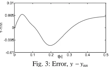
Fig. 3 shows the relatively small error between these step responses.

Fig. 3: Error, y ynn

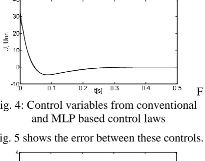
F ig. 4: Control variables from conventional

and MLP based control laws

Fig. 5 shows the error between these controls.

Fig. 5: Control error, u unn

It is important to realise that the errors shown in Table 1 are only for the training points while the errors of Fig. 5 indicate the interpolation ability of the MLP because the states presented to the MLP during the simulation are not the same as those presented to it during the training.

These results demonstrate the success of the training process. The performance, of course, is affected by the accuracy of the approximation achieved during the training and this is monitored during execution of the Matlab MLP training software by means of the plot shown in Fig. 6 which displays the mean square error versus the training time (epochs). It is evident that the error decreases very rapidly to the acceptably small value selected as an input parameter of the software.

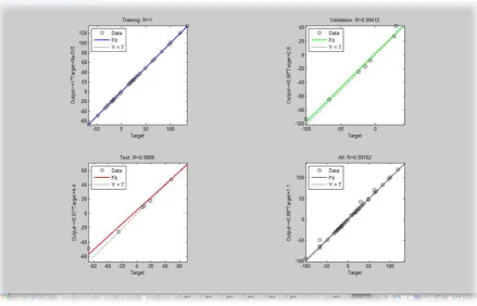
Fig. 7 shows plots from the training software for analysis of the network response with respect to training, validation, and test. The task is to put the entire data set through the

network and then perform the linear regression between the network outputs and the corresponding targets.

In this case, the outputs are tracking the target with acceptable accuracy and the R-values, i.e., the correlation coefficients, are:

Training=1, Validation=0.99412, and

Test=0.9898 with an average of R=0.99762.

3. Further observations:

It was found that the backpropagation with the gradient descent algorithm is generally very slow because it requires small learning rates for stable learning.

From the authors experience of previous simulations, it appears that networks are sensitive to the number of neurons in their hidden layers. Too few neurons can lead to

underfitting. Too many neurons can

contribute to overfitting, in which all the training points are well fitted, but the fitting curve oscillates wildly between these points.

4. Conclusions and

Recommendations:

The overall result shows that the MLP has been used to directly close the loop with a good approximation to the linear state feedback control law.

Since optimal control laws respecting control saturation constraints are nonlinear, the next step is to investigate the ability of the MLP to reproduce the well known time optimal state feedback control of a double integrator plant. Successful completion of this task will lead to the investigation of closed loop MLP control minimising the frictional energy wastage in an electric drive, the training data being generated from

optimal control calculations using

Fig. 6: Performance at 52 epochs showing that the target has been met

5. References:

Bellman R., Dreyfus S. E, Applied Dynamic

Programming, Princeton University Press, Princeton, NJ, 1962.

Bryson E. A., Ho Y. C., Applied Optimal

Control: Optimization, Estimation, and Control, Harvard University Press, Cambridge, Mass., 1975.

Matieni X., Dodds, S. J., Comparison of Fixed Final Time Optimal Control Computational Methods with the view to Closed Loop

Implementation using Artificial Neural

Networks, Proceedings of AC&T, University

of East London, 2009.

Pontryagin L. S., The Mathematical Theory of

Optimal Processes, I. The Maximum Principle, Izv, Akad. Nauk, SSR, Ser. Mat. 24, 3, 1960.

Ryan, E. P., Optimal relay and saturating

control system synthesis.-IEE Control Engineering Series, 1982

Dodds,,S. J., ‗Settling Time Formulae for the Design of Control Systems with Linear

Closed Loop Dynamics‘, Proceedings of

AC&T SCOT, University of East London,