Interactions Between Inflation, Monetary and
Fiscal Policy
Oscar J. Arce
PhD Thesis, Department of Economics
UMI Number: U61BB62
All rights reserved
INFORMATION TO ALL U SE R S
The quality of this reproduction is d ep en d en t upon the quality of the copy subm itted.
In the unlikely even t that the author did not sen d a com plete m anuscript
and there are m issing p a g e s, th e se will be noted. Also, if material had to be rem oved,
a note will indicate the deletion.
Dissertation Publishing
UMI U 613362
Published by ProQ uest LLC 2014. Copyright in the Dissertation held by the Author.
Microform Edition © ProQ uest LLC.
All rights reserved. This work is protected against unauthorized copying under Title 17, United S ta tes C ode.
ProQ uest LLC
789 East E isenhow er Parkway
L i D f b ? y
B ritish Library or Political
Abstract
In Chapter 1 I develop a simple model, that builds upon some previous work on
financial innovation processes, to account for the main stylized facts observed during
extreme hyperinflations. The modeling device used here helps to reconcile some
conflicting views on the causes, development and end of a hyperinflation without
departing from the rational expectations assumption. Specifically, it is shown th at the
effectiveness of a future orthodox reform to preclude the occurrence of a hyperinflation,
either speculative or fundamental, is an endogenous outcome which depends on a wide
array of policy choices (fiscal and monetary) and structural features of the economy.
In Chapter 2 I examine the postulates of the Fiscal Theory of the Price Level
(FTPL) under an interest rate peg. I show th a t the usual definition of a non-Ricardian
plan involves a non-credible government policy commitment, thus confuting the
interpretation of the FTPL as a policy-based equilibrium selection device. Then I
identify the set of necessary conditions for the implementation of non-Ricardian fiscal
plans th at result in a unique equilibrium. A critical necessary condition for the
credibility of a fiscalist plan is th at the equilibrium level of seigniorage must be non
positive. I argue th at the fiscalist stock-analogy is only meaningful, precisely, when
money enters into the government constraint as a destination of funds, rather than as a
source.
In Chapter 3, I extend Buiter’s (2001, 2002) criticism (non-Ricardian plans are
generally non-implementable whenever the monetary authority sets a non-contingent
sequence of money supplies) to an infinite horizon economy. In particular, it is shown
th at a fiscalist deflation involves the violation of a household’s optimality condition and
that the notion of a fiscally-induced speculative hyperinflation cannot be rationalized
invoking a symmetry between the problem of pricing a potentially fiat non-convertible
asset (like money) and that of pricing the stock of a private firm as advocated by the
Table of Contents
Acknowledgments... 4
1 A Model of Hyperinflations with Rational Agents and Orthodox Reforms... 5
1.1 Introduction...5
1.2 Stylized facts...1 1 1.3 A simple model with money-demand hysteresis... 13
1.3.1 The households...14
1.3.2 The government... 22
1.4 Equilibrium: Definition and characterization...19
1.4.1 Equilibrium and individual behavior... 19
1.4.2 Inflation dynamics: Some extra assumptions...2 0 1.5 Results...23
1.5.1 Hyperinflationary paths: The case of an ineffective reform... 25
1.5.2 The relative role of expectations and fundamentals... 29
1.5.3 Some numerical illustrations... 37
1.5.4 State-contingent reforms... 39
1.6 Concluding remarks...44
Appendix... 46
2 The Fiscal Theory of the Price Level: A Narrow Theory for non-Fiat Money... 55
2.1 Introduction...55
2.2 The canonical non-Ricardian argument... 59
2.2.1 The model... 60
2.2.2 Ricardian and Non-Ricardian policies...62
2.3 The role of transversality conditions...6 8 2.4 The limits of well-defined non-Ricardian policies...76
2.4.1 Ruling out government supersolvency...77
2.4.2 The asymmetry between government default and supersolvency...80
2.4.3 The necessity of convertible (non-fiat) money... 82
2.5 Learning from the fiscalist stock-analogy... 85
2 . 6 A multiple-period economy...90
2.7 Conclusions... 96
3 On Fiscalist Divergent Price-Paths... 99
3.1 Introduction... 99
3.2 Monetarist discipline vs Fiscalist laissez-faire... 103
3.2.1 A simple model...103
3.2.2 Ricardian vs non-Ricardian...106
3.3 Fiscalist speculative deflations: An issue of rationality...1 1 2 3.3.1 A cash-less economy...114
3.3.2 Introducing money... 116
3.4 Fiscalist non-deflationary paths: Not everything works... 120
3.4.1 A finite-horizon economy: Buiter’s criticism...1 2 2 3.4.2 An infinite-horizon economy... 123
3.4.3 Speculative hyperinflations: A necessary result?...127
3.5 Conclusions...133
List of Figures
Figure 1: Monetary base, seigniorage and inflation...49
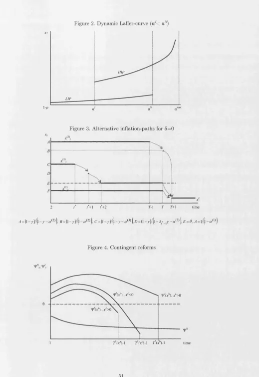
Figure 2: Dynamic Laffer curve... 51
Figure 3: Alternative inflation-paths for 5=0...51
Acknowledgements
Many ideas developed in the essays of this thesis have been shaped during my
interactions with Nobuhiro Kiyotaki to whom I am deeply grateful. Nobu is the best
supervisor and advisor I could have wished for. He always found time, listened and
gave lots of constructive comments. His generous patience and constant encouragement
were crucial to go ahead at those times in which I couldn’t see the end of the tunnel.
No doubt, being his student will continue to have a positive impact on my life in and
outside of economics.
I also thank Charles Goodhart, from whom I got much help during my first
steps at the LSE. I am grateful to both of them for their help in funding and job
search—th a t were essential for the completion of my studies.
Jose M. Martfnez-ScLnchez, from Universidad de Burgos, first suggested me to
undertake my graduate studies at a leading economics department. His advice and
constant help and support over these years are very much appreciated.
Many people gave valuable comments about my work, for which I am grateful:
Javier Andres, Gianluca Benigno, Paul Castillo, Tim Kehoe, Kostas Kofopoulos, David
Lbpez-Salido, Ben McCallum, Carlos Montoro, Fernando Restoy, Andrei Sarychev,
Javier Valles, Jesiis V&zquez, Jan Vlieghe, seminar participants at the LSE, Banco de
Espana, IX Workshop on Dynamic Macroeconomics, XIX Annual Meeting of the
European Economics Association, and XXIX Simposio de An&lisis Econ6mico. A special
thank you to Marco Bassetto for his comments on the second chapter.
Last, but not least, I want to thank the Banco de Espana for financing my
research. Their financial help while a graduate student was crucial for completion of
this thesis. Also the final part of this work was done while serving as an economist at
Chapter 1
A Model of Hyperinflations with
Rational Agents and Orthodox Reforms
1.1 In tr o d u c tio n
The general objective of this paper is to provide a theoretical explanation for the main
stylized facts observed during hyperinflationary processes, as those suffered by some Eu
ropean, Latin-American and transition countries in the 1920’s, 80’s and 90’s, respectively.
These episodes often display a common set of facts, yet much of the previous related liter
ature has followed a partial approach, concentrating on some of these facts but, critically,
neglecting others at the same time, as stressed by Bental and Eckstein (1990) and, more
recently, by Marcet and Nicolini (2003). Indeed, some of the most influential “partial
stories” , when combined together, yield a picture th at does not resemble what we actu
ally observe in real economies. A central contribution aimed here is to present a simple
rational-expectations general equilibrium model th at potentially accommodates three of
the most wide-spread partial approaches (the fiscal root, the bubble explanation and the
orthodox reform, briefly described below), making them consistent with each other and
with the empirical facts.
First, weak fiscal conditions th at force the government to finance a significant share
of the budget via money injections (seigniorage) are usually thought to be an important
factor behind hyperinflations (the fiscal root). In a general sense, this view is not refuted
by the empirical evidence since, on the one hand, explosive hyperinflations often take place
in countries in which seigniorage is relatively high and, on the other, a drastic reduction
in this source of funding is observed after every successful stabilization. For example,
regarding the fiscal stance of some European countries in the 1920’s, Sargent (1986; p.
45) observes that “the governments of these countries (Hungary, Austria, Poland, and
This was done on such a scale that it led to a depreciation of the currencies of spectacular
proportions.” (parentheses added)1. Although the exact intertemporal mechanisms linking
inflation and seigniorage are likely to be rather complex, as shown by Sargent and Wallace
(1981), the traditional proposition that associates high inflation to a high degree of fiscal
dominance in the implementation of monetary polices remains basically uncontested2.
Second, for some students of these episodes, the extremely high velocity taken by the
inflation rate over the course of a hyperinflation, without a noticeable change in the volume
of seigniorage, suggests th at these processes may well be driven just by expectations that,
in equilibrium, are self-confirmed (the bubble explanation). This approach has received a
formal treatm ent, under the rational expectations paradigm, among others, by Sargent
and Wallace (1987), and Bruno and Fischer (1990). Those authors assume a demand
for real balances a la Cagan3, which implies the existence of a hump-shaped inflation-tax
Laffer curve with two stationary inflation rates (one “low” and one “high”) associated to a
unique volume of seigniorage, and interpret a hyperinflation as the economy moving from
the vicinity of the low inflation rate to the high one. According to this view, seigniorage
is not the sole explanation for high inflation, instead, private expectations are thought to
be the prime cause. However, in explaining the occurrence of a hyperinflation as a bubble
equilibrium along a standard Laffer curve, the degree of fiscal pressure does no play any
significant role4. Still, such a possibility has also attracted much attention in the empirical
literature5. For example, Imrohoroglu (1993), provides empirical support for Sargent and
1 Sachs (1987) and Kiguel (1995) also point towards high levels of seigniorage as a prime cause in the hyperinflationary episodes in Bolivia and Argentina, respectively, in the 1980’s. Petrovic and Bogetic (1999) stress the massive resort to seigniorage as a key determinant of the violent hyperinflation suffered by Yusgoslavia in the early 1990’s. Reinhart and Savastano (2003) also share this view and provide some suggestive evidence on the size of the fiscal adjustments after the end of several recent hyperinflations.
2Yet there are some divergent views on this issue. For example, Loyo (2001) provides an explanation for the Brazilian several hyperinflationary bursts in the 1980’s and 90’s and assumes that the volume of seigniorage is negligible. Also, in the economy studied by Bental and Eckstein (1990), an upper bound on seigniorage is a necessary condition for the occurrence of the hyperinflation.
3 Much of the work undertaken in the hyperinflation literature, both theoretical and empirical, has been heavily influenced by the seminal work of Cagan (1956). In particular, Cagan assumes that the only changing argument in the demand for money is the expected rate of inflation, as a measure of the cost of holding money, an artifact intended to capture the fact that variations in other arguments of that function (e.g. the level of income and consumption, the real interest rate, etc.) are overwhelmed by the huge changes in the inflation rate over a hyperinflation.
4 More on the contrary, as the economy moves towards the decreasing arm of the Laffer curve, higher levels of seigniorage will result in lower inflation rates.
Wallace’s multiple-equilibria model using data from the German hyperinflation.
Third, for a wide class of rational-expectations economic models, including those in
the tradition of Cagan mentioned above, Obstfeld and Rogoff (1983) and Nicolini (1996)
have shown th at the prospect of a fiscal-monetary reform aimed at stabilizing the real
value of the currency (the orthodox reform) is itself a sufficient condition for precluding the
occurrence of a speculative hyperinflation, thus making it difficult to reconcile the idea of a
hyperinflation as a rational-bubble equilibrium. Moreover, once the possibility of a reform
is introduced in a model with rational expectations and a Cagan-style demand for money,
what one gets is th at higher levels of seigniorage are uniformly associated to more severe
disinflationary processes. As pointed out by Marcet and Nicolini (2003), if anything is
unambiguously true about hyperinflations is th at they are always stopped. There is little
doubt either th a t this is possible because of the government’s determination to reform
the fiscal-monetary mix, i.e. to implement “deliberate and drastic fiscal and monetary
measures taken to end the hyperinflations” (Sargent (1986; p. 44)).
Clearly, when combined together, these three partial views do not fit each other. Yet,
there have been a relatively few number of attem pts to provide a general theoretical
explanation for hyperinflations, including their causes, dynamics and end. To the best of
my knowledge, most of them consider models in which the preventive role of an eventual
reform, as the one outlined above, is not explicitly considered6. Marcet and Nicolini (2003)
consider a baseline model similar to the one studied by Sargent and Wallace (1987) but
assume th at individuals follow a backward-looking rule for forming expectations (quasi-
rational learning). They show that, under some conditions on the learning rule, the model
is able to match most of the stylized facts. However, as individuals do not internalize the
possibility of a future change in the policy-regime when forming their expectations, the
prospect of a reform is itself irrelevant for the dynamics of the model. Using the same basic
Cagan-type model, Kiguel (1989)7 argues that a volume of seigniorage above the maximum
one in a steady-state inflation-tax Laffer curve will unchain an explosive hyperinflation if
the money market does not clear instantaneously. Although he explicitly considers the
and Hooker (2000 and 2003).
6Drazen and Helpman (1990) provide an exception, for they explicitly model the effects of anticipated change of regime. However, in order for their model to generate a hyperinflationary path, an upward seigniorage-path is required, something that, as discussed below, is not a common feature in hyperinfla tionary episodes (see Bental and Eckstein (1990) for a discussion of this point).
implementation of a reform as a device to stop the hyperinflation, the expectation of a
reform does not have any effect on individuals decisions before its implementation either8.
The two models just mentioned provide a rationale for the fiscal root view, however at
the cost of neglecting the course of the government actions executed beyond the current
date. A radically different view is taken by Bental and Eckstein (1990) and Paal (2000),
since in these models the anticipation of a reform is thought to be the cause of the
hyperinflation. Bental and Eckstein explain the relatively low level of monetization (i.e.
the stock of real balances) observed for a long time after the end of a hyperinflation
as a consequence of a negative wealth effect arising from the increase in income-taxes
accompanying a drastic fiscal-monetary reform. Then, they interpret a hyperinflation as
the economy moving from a scenario of a high demand for real money to a stationary one
in which, for any given inflation rate, the stock of real balances remains low, in line with
a lower level of private wealth. Paal (2000), referring to the hyperinflationary episode in
Hungary in the 1940’s, argues th at a reform based on the stabilization of the inflation rate
without directly controlling for a monetary aggregate may actually leave the economy
prone to purely expectational-driven equilibria, some of them hyperinflationary, some
others exhibiting a pronounced disinflation. Anticipation of such a change in the monetary
rule, rather than a weak government’s fiscal condition, could have been, according to this
model, the true cause of the Hungarian hyperinflation9.
The approach followed here may be seen as a complement to the “general” expla
nations listed above, for it shares some basic features with them, yet takes a different
route. I do not impose ex ante any special assumption on the current effects of a fu
ture reform. Rather, I am concerned with the conditions under which the prospect of an
eventual reform exerts a preventive effect. In this sense, I build up a framework within
which the effectiveness of a reform to preclude the occurrence of a hyperinflation arises
as an endogenous outcome. To this aim, I formulate a rational-expectations model whose
8 As observed by Kiguel, imposing a sufficiently tight limit to the speed of adjustment of the m oney market am ounts to transforming the dynamics of an otherwise standard rational-expectations m odel into the ones o f a model with adaptive expectations, an issue which is discussed later in more detail.
cornerstone is its potential ability to display one of the most recurrent empirical facts
in hyperinflationary economies, namely, a post-reform hysteresis-effect in the demand for
(national currency) real balances. Referring to this phenomenon, Calvo and V6gh (1992;
p. 1 1) note that “high inflation forces a gradual development of new financial instruments
[...] Creating new financial products is costly and requires a learning process. Once this
investment has taken place, the public will continue using these new financial instruments
even if inflation falls”10. Along this line of reasoning, the model developed later features
a gradual development of a non-monetary financial instrument whose initial adoption is
costly but th at can be used even if inflation falls. There are several theoretical models in
the previous literature designed to account for some of these facts. For example, Ireland
(1995), Sachs (1995) and Uribe (1997) all provide examples of economies in which a form
of financial innovation exhibits long-lasting effects. However, to my knowledge, no model
of financial innovation or currency substitution has been previously exploited to account
for the stylized effects we are after, including an explosive inflation-path and a sudden
change of policy-regime. Thus, a methodological contribution of the paper consists in
bringing together these two strands of the literature, a natural step after recognizing
th at the incentives to invest in financial products not directly subject to the inflation-tax
are probably highest when inflation reaches several-digits values, and th at the most pro
nounced episodes of rapid demonetization and slow remonetization are observed during
hyperinflationary episodes11.
Specifically, I model the demand for monetary balances as a version of Ireland’s cash-
and credit- goods environment. Private individuals may acquire their desired consumption
basket by using either cash or credit. However, the usage of credit requires the prior
investment of some valuable resources for building up long-lasting credit relationships
which can be exploited for some time to avoid the inflationary cost of carrying cash12. On
10A similar observation can be found in Dornbusch et al. (1990; p. 23-24): “The distinction between movem ents along the real money demand schedule and shifts in real m oney dem and helps explain the actual dynamics of real balances during an inflation. The distinction m ay also explain why there are hysteresis effects. Once a new financial product is in use, it will continue to be used even if inflation declines. [...] Financial institutions are not ready-made to accommodate the flight from money. In the short run, households m ay hold more real balances than they will after alternative vehicles become available or better known. In practice, this will look like adjustm ent lags, but it also reflects the adjustm ents of financial institutions to the increased inflation."
11 The possibility of employing a model of gradual financial adaptation to account for the stylized facts observed in hyperinflations was first suggested by Uribe (1997), although he limited his analysis to steady-states characterization. This paper can be viewed as following up on his observation.
the side of monetary supply, I follow the standard assumption of a government aiming at
collecting an exogenous and constant amount of seigniorage over a fiscal-dominance regime
which is possibly reversed at some future date by the implementation of a monetary-fiscal
reform conducive to a low-inflation monetary-dominance regime13. Private agents are
assumed to be aware of the eventual change of regime. Such a simple formal apparatus
turns out to provide a natural interpretation on the possible links among the fiscal roots of
the hyperinflations, their dynamics and termination and the relative role of expectations
and fundamentals. In particular, provided some mild conditions hold, the model exhibits
up to three general classes of potential equilibria over the fiscal-dominance regime. First,
a unique low-inflation equilibrium th at arises when the public expects a “responsible”
government policy in the form of a combination of a low level of deficit-monetization
and an early and restrictive reform. Second, a unique high- and increasing-inflation path
th at obtains in the opposite policy scenario (i.e. high seigniorage and late/insufficiently
restrictive reform). Third, for some structural parameters and government policy choices
lying in between the two previous extreme cases, the model displays multiple equilibria,
some of them hyperinflationary, whose realization hinges crucially on private expectations,
this being a reflection of the fact th at a seigniorage-based monetary policy allows per se
for individual complementarities in the decision of investment in the credit-technology.
Overall the main insights of the paper are two. First, on the theory side, the paper
argues th at the practical relevance of the strong arguments put forward by Obstfeld and
Rogoff, concerning the effectiveness of a future reform to rule out a hyperinflation, must
be qualified in view of the empirical evidence, for the presence of hysteresis suggests th at
the sufficient condition for the validity of those arguments (i.e. the lack of causality run
ning from past to future states along an equilibrium in which the prospect of a reform
is internalized by the households) may not hold in real economies. Indeed, in an econ
omy in which hysteresis is a true possibility, the conditions under those arguments hold
are likely to be much more complex than in the history-independent economy studied by
on the use of domestic money (e.g. dollarization, barter, etc.)
those authors. This observation will allow us to reconcile the three influential views on
hyperinflationary processes described above. Second, by examining the necessary and suf
ficient conditions for a hyperinflation, the model offers some insights potentially relevant
for policy judgment. In particular, fiscal conditions are likely to play an important role, as
stressed by Marcet and Nicolini (2003). However, using a genuine rational-expectations
dynamic framework, we learn th at seigniorage over the fiscal-dominance regime, while im
portant, does not contain all the relevant fiscal-information, e.g. the horizon over which
that regime is implemented and the fiscal-monetary conditions prevailing after the re
form are also likely to have a direct effect on the conditions th at determine whether a
hyperinflation is a feasible outcome or not.
The rest of the paper is organized as follows. Section 1 . 2 describes the main empirical
facts observed in a variety of hyperinflations. Section 1.3 contains the model. Section
1.4 characterizes the equilibrium conditions and introduces and discusses some general
assumptions on the model’s parameters. Section 1.5 contains the main results of the paper,
dealing with the conditions under which hyperinflations (speculative or “fundamental”)
are possible equilibrium outcomes under two alternative reforms (contingent and fixed-
date reforms). Section 1.6 summarizes the main results of the paper.
1.2 S ty liz e d fa c ts
Over the course of the last century and until very recent times a considerable number of
countries have experienced episodes of vertiginous falls in the value of their currencies.
Some of these episodes are so distant in time and/or geographical location th a t a detailed
list of the economic factors underlying each single hyperinflationary is just an unfeasible
task. Nevertheless, the literature has in most cases come to agree on a number of stylized
facts th at have been present in virtually all the hyperinflations occurred so far. Below, I
briefly describe those facts14.
F irst Hyperinflations usually occur in countries experiencing important fiscal imbal
ances, in the sense th at the volume of resources th at the government is able to collect
from regular taxes and borrowing from (national or international) financial markets is,
on average, significantly below the level of its obligations, so th at the resulting difference
is funded by printing money (i.e. seigniorage). Fischer et al. (2002) report a strong
positive relationship between seigniorage, deficits and inflation using annual observations
corresponding to a sample of 24 high-inflation countries over the period 1960-199515.
Second. Real balances fall as inflation increases over the course of a hyperinflation.
Third. When inflation reaches its highest values within the hyperinflationary episode
there is a lack of strong contemporaneous correlation between seigniorage and inflation.
Indeed, seigniorage may well decrease significantly while inflation still grows at increasing
rates16.
Fourth. Stopping a hyperinflationary process usually involves a mix of fiscal and
monetary reforms whose aim is to set limits to the ability of the government to monetize
its deficit by e.g. setting government expenditures at levels according with its capability to
cover them by taxation and debt emission, fixing the exchange rate to a foreign currency
with a good reputation in terms of inflation, establishing legally independent central banks
with limitations to the amount of funds to be let to the government, implementing rules
to keep the growth of the money supply under limits (e.g. through currency boards), etc.
The process of inflation-stabilization (from the peak of the inflation series to the, usually,
stable and low rate after the monetary reform) takes a short period (two or three months
at most).
Fifth. The demand for real balances remains low, but exhibiting an upward trend,
for a long period after the stabilization17. This hysteresis-effect is behind the well doc
umented observation that, just after the stabilization, (nominal) money supply increases
at moderate-high rates without causing noticeable inflationary pressure.
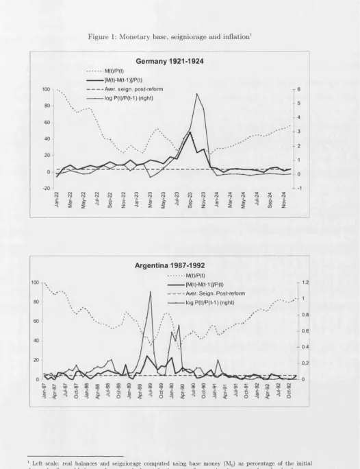
Figure 1 contains some empirical evidence on several hyperinflationary episodes recorded
in Germany, Argentina, Bolivia and Peru. These data generally confirm the “standard”
facts above. In all cases, the rise in inflation goes parallel to the fall in real balances. The
15For another recent survey on this issue, see also Catao and Terrones (2005).
16 The absence of a marked trend in seigniorage during hyperinflationary periods has led many re searchers to model this variable as a constant (or w ith a constant mean, in stochastic environments). This is the strategy followed by e.g. Bental and Eckstein (1990), Bruno and Fischer (1990), Kiguel (1989), Marcet and Nicolini (2003), Paal (2000) and Sargent and Wallace (1987). The model presented here uses this simplifying assumption too.
peaks in the inflation rate uniformly go together with the lowest value of the stock of real
money recorded for the entire period. At th at point the stock of real balances falls bellow
the 40% of its value a couple of years before. Although average seigniorage is clearly
higher in the pre-reform period than after the collapse of the hyperinflationary path for
the four countries, in some cases inflation reaches its highest value while seigniorage is
clearly decreasing (as in Germany 10:1923 and Bolivia 12:1984-2:1985) while in others
seigniorage remains high and increasing (as in Argentina) or fairly constant (as in Peru).
In all cases, after the stabilization, the volume of seigniorage was drastically cut down,
inflation remained low and stable, and the stock of real balances exhibited a very slow
recovery, thus confirming a strong hysteresis-effect.
1 .3 A s im p le m o d e l w ith m o n e y -d e m a n d h y s te r e s is
The model developed in this section is inspired in the cash-and-credit transactions econ
omy studied by Ireland (1995), who extends the Lucas and Stokey’s (1987) framework to
allow for persistent effects in the use of credit. Households are assumed to exchange their
consumption-goods endowments by using government-provided money or interpersonal
credit. The latter form of trade requires the existence of a credit-contract between the
intervening parts. Creation of such a contract involves some initial fixed and irreversible
cost. However an existing contract can be used at not further cost at any subsequent date
on which the contract remains operative. Transactions made using money do not carry
over any explicit cost beyond th at associated to the erosion of the real value of money
due to inflation. The main difference with respect to Ireland’s model is intended to keep
the subsequent dynamic analysis as simple as possible18. In particular, I assume th at the
volume of investment in the credit technology in any period is bounded above, as the
opportunities for investment in the credit technology arrive at a finite rate. This artifact
allows us to focus on monetary regimes along which the government is able to extract an
exogenously set amount of seigniorage over a non-trivial number of periods.
1.3.1 T he households
Consider a discrete-time economy with N (> 3) types of goods and N types of households
of population size 1 /N each. The household of type j produces goods j and consumes
goods j + 1 (except the one with type N who consumes good 1). Each household consists
of a continuum of members of unit mass. Half of the members within a household are
producers, who can produce their goods up to a given capacity y without cost. The other
half are buyers, without such a production capacity. All the members in a household share
consumption equally. At each date t, a fraction n3 of household-j’s members, producers
and buyers, are linked to the credit system, while the remaining fraction 1 — n3 are
not. Each linked buyer has an established bilateral relationship with a producer to buy
her consumption goods c^3 through a credit-contract, subject to the capacity constraint
cct’3 < y. Symmetrically, each linked producer has a bilateral relationship with a buyer to
sell his product C^'3 < y on credit. All non-linked buyers (producers) go to a centralized
market to buy (sell) goods with (in exchange for) cash as anonymous members. Money
received by non-linked producers cannot be passed to buyers within the same household
until the beginning of the following period.
The timing of events is as follows. At the beginning of every period t > 1, households
convene in the centralized financial market to settle outstanding debts and to accumulate
government-issued money and bonds. Both government and private debts mature one pe
riod after issued and pay the same nominal risk-free rate. Household-j enters this market
with the cash obtained from selling a part of the common endowment at t — 1, denoted
by M 3_ ±, with some maturing government bonds, inclusive of interest, ( 1 + it- i) ^ _ 1?
some invoices over other households, corresponding to the amount of goods sold on credit
during last period, ( 1 + it- i) P t - i C ^ and, symmetrically, some debts corresponding to
last period’s credit-financed purchases, (1 + it- i) P t-ic ^ iv The terms B 3_ ±, Cjzfj, c ^ 1?
it- 1 and P t-i axe, respectively, bond holdings, invoices over last period’s sales and pur
chases of goods on credit (measured in real terms), the nominal rate and the general price
level19. The government participates in this market redeeming maturing bonds, collecting
seigniorage (i.e. money injections by the central bank) and taxes (assumed to be paid in
cash) and issuing new bonds.
The household’s constraint in this market is
M i + B{ + Ptr t < M U + (1 + i t -1) ( 4 . , + C & - C & ) = W i (1.1)
where 7 7 is the lump-sum tax and M / j is the household’s stock of monetary balances at
the end of the previous period and, hence, it satisfies M{ > ( i- » 0 Pty. Households are
precluded from issuing money, i.e.
M{ > 0 (1.2)
Once the households rearrange their portfolios of money and bonds, non-linked producers
engage in a process of finding buyers for their goods to sign a credit-contract. A free
producer finds an opportunity to establish a credit link with a buyer with a given prob
ability 7 < 1. In such an event, the producer may chose to sign a contract by paying a
utility cost of O20. In th at case, the buyer commits to redeem the resulting debt, plus the
interest rate, in exchange for money at the financial market during the following period.
Clearly, imposing 7 < 1 tantamounts to a limit on the speed of investment in the credit
technology which, as seen later in detail, translates into an upper bond to the speed of “de
monetization” . In other words, it implies th at building up a certain stock of credit-links
takes time21. In a symmetric vein, as in Ireland (1995), I assume th at the households’
credit capacity is subject to a form of depreciation. In particular, credit-contracts have,
on average, a finite life, as they are subject to a constant probability of termination at
the beginning of each period equal to 822. This assumption is critical for the arguments
developed later. In practical terms, it implies th a t current individual decisions on the mix
of money and credit used to carry out transactions may have effects beyond the current
20 A contract will generally create some “monopolistic” rents for the counterparts. As the main interest here is in the evolution of the aggregate stock of credit-contracts, real balances and, in turn, inflation, I consider a very simple (and extreme) rule governing the sharing of the benefits arising from a match. In particular, I assume that the seller pays the fixed utility-cost and leaves the buyer only with an infinitesimal share of the monopolistic pecuniary rents of the contract. As participating in a contract is costless for the shopper, she is happy to accept any strictly positive payment. For notational simplification, I omit that negligible transfer in the forthcoming expressions.
21 The assumptions of a constant probability of arrival of a credit-link opportunity and the symmetric proportion of linked producers and buyers are compatible with a random matching framework in which each individual can only commit to maintain a single credit-link and the matching function exhibits constant returns to scale in the number of non-linked agents on both sides of the market and a linear time-invariant total-efficiency parameter 7 .
date and, hence, it works as a simple device aimed at capturing the presence of hysteresis
in the demand for money observed after hyperinflationary episodes.
Notice that, while there is uncertainty at the individual agent level, the assumption
of a continuum of agents within each household implies th at at the household level, there
is no uncertainty on the total measure of the flows of new and existing contracts. Thus,
the law of motion of the measure of credit-linked producers within household-.? can be
expressed as23
n3t = 7 1 - (1 - 5) Af + (1 — 5) n\_ x (1.3)
where the parameter X3t captures the proportion of producers th at do take advantage of
an opportunity to create a credit link, and, hence, it satisfies \ j € [0,1].
Then, the centralized market for goods opens. In this market, producers who do
not deliver their stock of goods through a credit arrangement sell their endowments in
exchange for money. Here, the following standard CIA-constraint applies,
cT J < ^Ft (1-4)
where q™'3 refers to the total measure of goods consumed by j that are purchased with
cash. Finally, the members of the household join to consume the buyers’ purchases. In
making its choices at t, the household must respect the following flow of funds constraint
W 3t+1+ i tM 3
+ Pt (c?'3 + < P t { y - Tt) + W 3 (1.5)
1 + H
and a borrowing constraint th at rules out games & la Ponzi
lim W y ( 1 -I- it) > 0 (1.6)
oo t=i
All households enter period 1 with the same financial wealth, in an amount exogenously
given, i.e. W{ = W \. Also, the measure of credit-linked producers at the beginning of
period 1 (just before the destruction of some of these contracts) is given by history and
identical for every household, i.e. n30 = uq.
Household-j chooses a path for M i.-- .---- , M i ,B 3s , n i , \ J3 >. 'I CXJ in order to maximize s = t
Ut = £ p r ' {in 4 - 07 [l - (1 - <5) n j ,,] A^} (1.7)
S= t
where d = c™’J -I- CsJ , subject to the set of constraints in (1.1), (1.2), (1.3), (1.4), (1.5),
and (1.6).
1.3.2 T he governm ent
The government in this economy collects taxes, issues and redeems bonds and provides
the entire stock of money. When choosing a particular combination of policy-instruments,
the government is restricted by the two following constraints. First, a period-by-period
flow of funds constraint,
where Mt and Bt represent the government supply of money and bonds at t, respec
tively. Government consumption is assumed to be set at zero at every date. Second, an
intertemporal constraint, given by
f i i „• a d Pt+sTt+s + M t+S ~ Mt + S - 1
(1 + I t -1) B t-1 = 2 ^ ffs 77—1 X (1-9)
fri
1 I z = i ( ! + * * + / )I assume throughout that the government targets a constant (and finite) real-valued stock
of end-of-period outstanding bonds, i.e. ^ ^ for t > 1, with > 0 being exogenously
given by history. Regarding monetary policy, I consider two alternative policy regimes.
During the first regime, operating from period 1 to T > 1 (including both), the government
sets an exogenous target for seigniorage. Money supply is then adjusted to satisfy a
seigniorage requirement, denoted by a, according to the following rule
A second monetary regime is implemented at T + 1 (this date is henceforth referred as the
tion rates by adjusting money supply accordingly. For notational simplicity and without
Bt + M t
~ pT ~ t =
( 1 + it~ i) B t~ i + M t~i
Pt (1.8)
M t = Pta -I- Mt - 1 (1 < t < T) (1.10)
infla-loss of generality, I assume th at the targeted level of inflation under this regime is con
stant, denoted by x L. As, in principle, the model admits multiplicity of equilibria under a
targeted-inflation monetary rule, some of them hyperinflationary, it is also assumed th at
the government is willing to respond to upwards deviations from the target by backing
the stock of money according to the following strategy. Taking Pt and the aggregate
equilibrium stock of money at th at date, Mt, as given24, the government announces a
sequence of money supplies {M t}^.T+ i. Such a sequence of money supplies will map into
a unique sequence of equilibrium inflation rates if and only if the demand for real balances
and, hence, the price level follow a unique path from T + 1 on. Let’s denote this sequence
of non-hyperinflationary prices as { ^ P} ^ T+1, whose exact elements are understood to
p G
depend on {M t}^.T+ i, Mt and Pt, and satisfy ff+g1 — 1 = x , for s = 0,1,..., oo. Then,
in view of an arbitrary price Pt > P f1 at any t > T + 1 , the government reacts by offering
the households the possibility of redeeming each monetary unit in exchange for bonds,
where < Pt < Pt- Such a deal creates an arbitrage opportunity which cannot be com
patible with individual optimization and, hence, any Pt above the one consistent with the
government’s inflation target cannot be part of an equilibrium25. Notice th at for such a
backing-scheme to be effective it must be credible, in the sense th at the households expect
a current and/or future fiscal adjustment consistent with the endogenous higher supply
of government bonds. Specifically, credibility of this government’s contingent strategy
requires the commitment to increase the total discounted value of taxes by an amount
equal to
As shown later, in most cases, after the reform there will be a upward adjustment in
the demand for real balances. Thus, a constant targeted x L over this regime will require
money injections, i.e. M t > Mt~i for t > T +1, which in turn implies th at the government
will earn some seigniorage whose amount is (endogenously) driven by the path followed
by the stock of real balances. Therefore, in this regime, for a policy of zero government
consumption and constant stock of debt, taxes must adjust endogenously so as to satisfy
(1.8) and (1.9). From now on, I will refer to the two policy regimes described above as
fiscal-dominance (for 1 < t < T, i.e. the pre-reform period) and monetary-dominance
regimes (for t > T + 1, post-reform period).
24Notice that, given the money supply rule followed up to T (inclusive), the stock of money at that date is not direclty targeted by the government.
1 .4 E q u ilib riu m : D e fin itio n a n d c h a r a c te r iz a tio n
In this section I state the definition of equilibrium used in the remaining, describe the
solution of the representative household’s maximization problem and introduce some as
sumptions regarding several classes of dynamic paths followed by the endogenous variables
of greatest interest (the demand for real balances and the inflation rate).
1.4.1 Equilibrium and individual behavior
Henceforth, I will focus on symmetric competitive equilibria for the economy just de
scribed26, defined according to
D efinition 1 A perfect-foresight symmetric competitive equilibrium in this economy is a
collection of sequences { c™, <?s, Ms, M s, B s, n s, Xs, Ps, is j and a government policy such
f J s = t
that the following conditions are satisfied:
1. Households maximize their utility subject to the initial conditions, W \ and no, and
the constraints (1.1)-(1.6), taking as given the price and interest rate sequences and the
government policy.
2. The government satisfies its budget constraints (1.8) and (1.9).
3. All markets clear at each date.
The following conditions are necessary and sufficient for characterizing the optimal
individual behavior:
1) The intertemporal allocation of consumption satisfies the Euler equation
^ = /J (l + i , ) £ - (1.1 1)
ct Ht+i
2) When facing an opportunity, a producer decides to establish a credit link and pay
the fixed utility-cost if > 9, it is indifferent if \I/t = 6 and does not sign the contract
otherwise. The shadow-value function S&t captures the discounted sum of the expected
savings, in terms of the inflationary tax, delivered by a credit-link, and is given by
i (i - a r 1
n?=o (i +**+<) p,+t+i
®‘ = ^ - 1 . - \ K . <L12)
where Xt+i is the inflation rate between t and t + 1, i.e. — 1 and <f>is an indicator
function capturing whether the producer is using th at credit-contract at each date. It
takes two values: 1 if the producer uses th at link and 0 otherwise. In writing (1.12), we
note th at the effective inflation-savings from signing a contract at t is the discounted sum
of the product of the inflation rate times the amount transacted via credit. Notice th at
the discount factor used here takes into account the expected lifetime of the credit-link,
as captured by 1 — 8.
3) The producers of the household optimally decide to use of every existing link if
xt+i > 0 (thus setting 4>t = 1), they are indifferent between transacting using the credit
facility if xt+i = 0 and decide to trade their endowments in exchange for cash if Xt+i <0
(fit = 0).
4) As long as27 it > 0 bonds perform better than money as an instrument for saving,
so th a t the household optimally decides to minimize its end-of-period money holdings,
i.e. y f = 0? and ^ = ( 1 - n t- i ) y.
5) When behaving optimally, the household does not leave any intrinsically valuable
resource unconsumed. Thus the flow of funds constraint (1.5) and the transversality
condition (1.6) hold as equalities.
1.4.2 Inflation dynam ics: Som e extra assum ptions
Before characterizing the main results of the paper, it is helpful to state explicitly some
equilibrium results and to describe the evolution of the endogenous variables of the model
under alternative kinds of (potential) equilibria. In this section I first solve for some
alternative equations governing the dynamics of the aggregate demand for real balances
and inflation as functions of the parameters of the model over the fiscal-dominance regime
and then I introduce some assumptions concerning the volume of seigniorage collected in
th at regime.
Henceforth, I will mainly focus on those cases in which the households either exploit
the possibility to establish a credit-link whenever possible (At = 1) or refuse to invest in
the credit technology at all28 (At = 0). Assuming the former case, At = 1, the overall
economy measure of producers with a credit-link at £, according to (1.3), is given by
nt = 7 + (l —7 ) ( 1 —5)n t_ i (1.13)
Thus, the proportion of producers th at sell their goods in exchange for money can be
written as
mt = (1 - 7 ) [1 ~ (1 - $) (1 - m t-1)] = (t > 1) (1.14)
After applying the normalization y — 1, from the equilibrium condition Mt = M t, it
follows th a t m t above represents the end-of-period stock of real balances in the economy.
As long as ft > 0, m t may take values in the unit interval.
Equation (1.14) captures the law of motion of m conditional on every producer invest
ing in the credit technology at the highest pace. Conversely, when no new credit-links
are made, i.e. At = 0, it can be readily verified th at the degree of monetization evolves
according to
m t = 1 - (1 - 6) (1 - m t-1) = TN (m*_i) (t > 1) (1-15)
Next, I introduce the following general assumptions.
(Consistency with the assumption of exogenous seigniorage) The level of seigniorage
collected over the fiscal-dominance regime, a , is bounded above by
a < a max = S( 1 — 7) b?7r - 1 rao (1-16)
I — 77
where 77 = (1 — 5) (1 — 7). When this inequality holds, the amount of seigniorage targeted
by the government before the implementation of the reform is feasible even when every
household invests in the credit technology in every period 1 < t < T — 1, so th a t m x - i
takes its minimum possible value (given by the RHS of (1.16)).
(Dynamic negative association between real balances and inflation). For 5 < 1, the
targeted level of seigniorage satisfies
a > 8 (1.17)
This condition implies that, regardless of the evolution of the degree of monetization at
every t € [2, T ] , i.e. whether mt follows (1.14) or (1.15), the resulting inflation rate, xt,
is a negative function of the last-period degree of monetization, m t -1- To see this, let’s
write (1.1 0) as
Xt = m t~1 - 1, 2 < t < T (1.18)
m t — a
Then, substituting m t for its two extreme values given in (1.14), T1 (m t~i), and (1.15),
(m t~i ) , and taking a simple derivative in (1.18), we can write
d x t d mt - 1
d x t dmt - 1
< 0 a > 5 (1 — 7 )
m t = r T(mt-i)
< 0 o l > 8
mt= r N (mt-i)
Thus, as 7 < 1, the inequality in (1.17) is a sufficient condition for the inflation rate to be
negatively related to m t -1, regardless of the law of motion followed by mt. This simple
observation will turn out critical in the analysis of the feasibility of hyperinflationary
paths in the next section. For the moment, it is useful to state the following result, which
is a direct consequence of the inflation-generation process (1.18) and the specification of
the T-functions, (1.14) and (1.15).
Given 8 < 1, if (1.17) holds, then the following equalities are satisfied
x{ > x ^ for 2 < t < T
x t+ 1 ^ x t and x t+ 1 < x t^ f°r 2 < t < T — 1
where x{ is the inflation rate satisfying (1.18), conditional on m s satisfying m s = T1 (ns-1),
for s = 2,..., t. Analogously, x ^ is defined as the inflation rate at t conditional on no credit-
link being established at any date from 1 up to t, both inclusive, i.e. m s — TN (m s-1), for
s = 2,..., t. Thus, it follows that, for a sufficiently high level of seigniorage, the inflation
rate associated with a sequence of degrees of monetization satisfying m s = T7 (ms_ 1) is
always higher than the corresponding to a sequence obeying m s = TN (m 3-1). Also, from
decreas-ing m-sequence is associated with an increasdecreas-ing sequence of inflation rates and vice versa,
i.e. increasing m over time leads to lower inflation rates29.
Thus, the basic economic message contained in the above result is a very simple one: by
restricting the volume of seigniorage to satisfy (1.17), we focus on fiscal-dominance regimes
along which a higher degree of monetization is invariably associated with a lower inflation
rate30. This idea resembles the one underlying the analyses based on the interpretation
of seigniorage as a tax paid by money holders, along the lines of a standard hump-shaped
inflation-tax Laffer curve, in the sense th at a higher tax base (i.e. real balances or degree
of monetization) needs a lower tax rate (i.e. inflation) to yield the same total revenue
(seigniorage). In view of this reflection, (1.17) seems a natural ingredient in analyzing the
dynamics of this economy under the fiscal-dominance regime. Also, as (1.17) imposes a
lower bound on seigniorage or, alternatively, a lower bound on the degree of persistence
of the credit technology, 1 — 5, it is not at odds with the common view of high levels
of seigniorage being, at least in part, responsible for hyperinflationary processes and
with the empirical evidence presented before regarding the slow recovery in the degree of
monetization observed after the end of the hyperinflations.
1.5 R e s u lts
In this section I check the ability of the model developed before to match the empirical
facts listed earlier and to provide an answer to two of the most recurrent questions in the
previous literature on hyperinflationary economies:
F ir s t. When is a credible fiscal-monetary reform effective to prevent a hyperinflation?
Second. What are the factors that may explain the occurrence of a hyperinflation as
a self-fulfilled prophecy?
I order to make the above qualitative queries explicit within the formal apparatus of
the model, it is convenient to give a meaning to the terms “hyperinflation” and “self
fulfilled hyperinflation” using the own language of the model. For this purpose, an impor
29 This statement depicts situations in which the degree of m onetization is not constant over the fiscal-dominance regime, i.e. it either increases or decreases monotonically over time. In the special case in which the initial condition, mo, happens to be equal to the stationary value of m under the corresponding law of motion, the degree of monetization remains constant over this regime and, hence, the inflation rate is constant too. The stationary values for m under the two law of motions (1.14) and (1.15) are, respectively, and 1.
tan t part of the following discussion is referred to two possible equilibrium inflation paths:
the highest inflationary path and the lowest inflationary path (HIP and LIP, henceforth).
Using these two concepts (whose formal definition is given below), I will henceforth use
the term “hyperinflation” as the occurrence of the HIP and “self-fulfilled” or “specula
tive” hyperinflation as the occurrence of the HIP whenever the LIP is, simultaneously, a
possible equilibrium outcome. On the one hand, this particular convention sacrifices some
generality. First, because, for a class of reforms (non-contingent or fixed-T reforms), on
purely empirical grounds, it might be difficult to distinguish the HIP from other possible
equilibria that yield inflation paths almost as high as the HIP. Second, because several
inflationary paths may coexist as potential equilibria with the LIP and/or the HIP or
other intermediate paths, so th at could equally be labelled as self-fulfilled inflationary
prophecies. On the other hand, by focusing on the conditions under which the HIP may
occur we will draw an important and interesting conceptual line, namely th a t one sepa
rating an “effective” fiscal-monetary reform (to be clarified later) from an irrelevant one.
This distinction turns out to be critical when analyzing contingent reforms (e.g. reforms
whose implementation hinges on the value taken by the inflation rate). Also, restricting
the analysis of the existence of self-fulfilled hyperinflations to situations in which these
two extreme kinds of inflation paths may arise facilitates the comparison of the results
yielded by this model with some more traditional approaches on the existence of multiple
equilibrium inflation paths, along which it is thought th at the same level of seigniorage
can be obtained at either a low and stable average inflation path or alongside an explosive,
ever-increasing, one. Nonetheless, the formal discussion th at follows also devotes some
attention to other non-extreme inflationary paths, in part because it is shown th at under
some conditions, non-extreme paths are the only possible equilibrium outcome.
In the remaining of this section, I first explore the conditions under which the HIP
may occur, assuming th at the government credibly commits to reform its fiscal-monetary
plan at some future date T -1-1, regardless of the state of the economy at th at date31.
Maintaining the assumption of non-contingent reform, I then investigate analytically the
conditions th at tend to favor the existence of speculative hyperinflationary paths (i.e.
situations in which both the HIP and LIP can be simultaneously supported as equilibrium
outcomes) and then perform some numerical simulations of the model. Finally, I explore
the determinants of the (in)effectiveness of an alternative state-contingent reform.
1.5.1 H yperinflationary paths: T he case o f an ineffective reform
Let’s suppose th at the government credibly commits to implement a reform as the one
described in section 3.2 at some date T + 1 and regardless of the state of the economy at
th at time. Also, to make life interesting, let’s assume that, independently of the history of
this economy up to T, the inflation rate targeted in the post-reform monetary-dominance
regime, x L, is bounded above by32
x L — xt+s < min < x t, — —--- --- -^r \ , s > 1 (1-19)
This inequality implies, first, th at the change of regime always leads to a fall in inflation
at the time of the reform, regardless of the history up to that date, and, second, th at
the reform always eliminates the individual incentives to reduce the usage of money, i.e.
the reform is successful in stopping an “eventual flight from money” from the time of its
implementation on, i.e., in equilibrium \ 3 = 0, s > T.
Assuming (1.17) holds, I define the two extreme paths (HIP and LIP) using the laws
of motion for the degree of monetization under the assumption th at At takes one of the
extreme values, 1 or 0, obtained before, (1.14) and (1.15), respectively.
D efinition 2 The highest inflationary path (HIP) is the sequence {x l}^ =2 that satisfies
(1.18) given that the sequence { m j^ 1 satisfies m t = Tr (m t-1) • The lowest inflationary
path (LIP) is the sequence that satisfies (1.18) given that the sequence
satisfies m t = TN (m t-1) .
Using the shadow-value function (1.12) together with the equilibrium conditions 1^ . ^ 1 =
/3- 1 and ct = 1, we can define the time-t (unique) shadow-value function associated to
the HIP as
T—t p f l1+1 /-i X\T—t
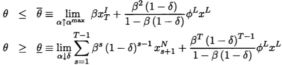
= E F t 1 - W ~ X *»+• + 1 - /? ( i - \) ^ (L20)
where (j)L G {0,1} denotes whether pre-existing credit-contracts are used after the re
form33. According to Definition 2, is given by
x , = (i
s( 1 - 7) TzJr + “ a
Thus, equation (1.20) captures the (gross) profit given by a credit contract when every
household exploits every opportunity for investment in the credit technology at each
single period within the pre-reform period (t = 1 ,...,T — 1). As the households follow
this pattern, provided a satisfies (1.17), the resulting equilibrium sequence of inflation
rates is the highest possible one. Then, denoting inf {'&t}^=i by and according to
(1.12), the following condition is necessary and sufficient for the feasibility of the HIP as
an equilibrium path34
¥ 4 > 0 (T2 2)
By simple inspection of (1.20) and (1.21), the qualitative effect of most parameters and
policy variables on condition (1.22) becomes apparent. Higher values of /? increase the
total return of the investment in a credit-link, thus raising \E^, and, hence, making
the HIP a more likely equilibrium outcome. Assuming (1.17) holds, a similar effect comes
from 5, as lower 8 means a longer average life for a contract. Also, from (1.2 1), higher
values 7 contribute to a more rapid demonetization and, thus, to a higher sequence of
future inflation rates and a higher value for the credit-technology at any t. This latter
effect is also caused by a lower initial condition, mo- From (1.20) and (1.22), it is also
clear th at a lower value for the cost of establishing a credit relationship, 6, tends to favor
the occurrence of the HIP.
Regarding the effects of the policy instruments, a , T and x L, their influence on con
dition (1.2 2) is also very intuitive. A high value of seigniorage goes in hand with higher
inflation rates, given a path for m, and with a higher &[. A restrictive monetary sup
ply over the post-reform period, contributes, given every thing else, to keep inflation low
also in the pre-reform period, since low values for x L reduce the expected return gained
33N otice that, since x L is time-invariant, the equilibrium value of (f>L will be constant too. As I will focus on situations in which inflation is striclty positive in the pre-reform regime, 4> will be optimally be 1 duirng that regime.
from each credit-link. Also, assuming (1.19) holds, an early reform (low T) reduces the
incentives to invest in the credit technology, since it shortens the period over which that
investment yields high inflation-savings (the pre-reform period). Finally, the effect of time
on i&t is likely to be non-monotonic, due to the discount-effect. Indeed, all the numerical
simulations discussed later yield a hump-shaped function, i.e. the lowest values for
are located at the beginning and at the end of the pre-reform period.
Thus, an equilibrium along which the prospect of an orthodox fiscal-monetary reform
does not have any positive effect on the demand for real balances and, hence, on the
inflation rate, except just at the moment of its implementation35, cannot always be ruled
out. This result is in clear contrast with the analysis of similar orthodox reforms carried
out by Obstfeld and Rogoff (1983) and Nicolini (1996), within the context of purely
forward-looking economies. In an economy like this one, in which past decisions of the
households have long-lasting effects, time matters. When this is case, the effectiveness
of a future reform to rule out explosive hyperinflationary paths hinges on the timing of
the reform, the monetary policy implemented in the post-reform regime (as captured
by x L) and also on the monetary stance before the reform (as captured by a) and on
some structural parameters of the economy governing the history-dependent processes
of demonetization and remonetization (as mo, S, 7 and 6). Also, when time plays a
non-trivial role, the concept of a static inflation-tax Laffer curve is no longer a useful
analytical tool, since whether