A comparison of fixed final time optimal control computational methods with a view to closed loop implementation using artificial neural networks

scroll down to view the document itself. Please refer to the repository record for this item and our policy information available from the repository home page for further information.

Author(s):Matieni, X. and Dodds, Stephen J.

Title: A comparison of fixed final time optimal control computational methods with a view to closed loop implementation using artificial neural networks

Year of publication:2009

Citation: Matieni, X. and Dodds, S.J. (2009) ‘A comparison of fixed final time optimal control computational methods with a view to closed loop implementation using artificial neural networks’ Proceedings of Advances in Computing and Technology, (AC&T) The School of Computing and Technology 4th Annual Conference, University of East London, pp.151-159

Link to published version:

A COMPARISON OF FIXED FINAL TIME OPTIMAL CONTROL 

COMPUTATIONAL METHODS WITH A VIEW TO CLOSED LOOP 

IMPLEMENTATION USING ARTIFICIAL NEURAL NETWORKS

 

X Matieni, S J Dodds

 

Control Research Group, SCoT. 

[email protected]; [email protected]; [email protected] 

Abstract:  The  purpose  of  this  paper  is  to  lay  the  foundations  of  a  new  generation  of  closed  loop  optimal  control  laws  based  on  the  plant  state  space  model  and  implemented  using  artificial  neural  networks.  The  basis  is  the  long  established  open  loop  methods  of  Bellman  and  Pontryagin,  which  compute optimal controls off line and apply them subsequently in real time. They are therefore open  loop  methods and  during the period leading up to the  present century, they  have been abandoned by  the  mainstream  control  researchers  due  to  a)  the  fundamental  drawback  of  susceptibility  to  plant  modelling errors and external disturbances and b) the lack of success in deriving closed loop versions  in all but the simplest and often unrealistic cases. The recent energy crisis, however, has promoted the  authors  to  re­visit  the  classical  optimal  control  methods  with  a  view  to  deriving  new  practicable  closed  loop  optimal  control  laws  that  could  save  terawatts  of  electrical  energy  by  replacement  of  classical  controllers  throughout  industry.  First  Bellman’s  and  Pontryagin’s  methods  are  compared  regarding ease of computation. Then a new optimal state feedback controller is proposed based on the  training of artificial neural networks with the computed optimal controls. 

1. Introduction:

 

After  the  establishment  of  classical  linear  feedback  control  theory  and  practice  in  the  1940s,  attention  was  turned  to  establishing  systematic  methods  for  adjusting  the  parameters  of  controllers  to  improve  their  performances,  leading  to  the  concept  of  minimising  (or  maximising)  a  performance  criterion  (Bellman,  1957).  Towards  the  end  of  the  1950s  and  during  the  1960s,  the  so  called modern control theory evolved centred  on  the  concept  of  the  state  of  a  dynamical  system,  which  proved  to  be  of  fundamental  importance  as  this  formed  the  foundation  stones of optimal  control  theory. One of  the  drawbacks  of  this  theory,  however,  is  that  closed  loop  versions  in  the  form  of  state  feedback  control  laws  offering  robustness  with  respect  to  external  disturbances  and  plant  modelling  uncertainties  are  not  readily 

attainable.  Such control laws, however, have  been derived for the time optimal control of a  limited range of plants (Ryan, 1982). 

The  structure  of  the  general  optimal  control  problem can be described as follows: 

a)  The plant or process to be controlled has  the following state space model:

( )

( ) ( )

( )

( )

 

, ,  ,

ì = é ù

ï _{ë û}

í

= é ù

ï ë û

î 

x x u 

y x 

&  t f t t t 

t h t t  (1) 

where x Î n  is  the  plant  state, u Î  r  is  the  set  of  control  inputs  and y Î  m  is  the  set of measured outputs. 

b)  There are restrictions on ( )u  t  and  ( )x  t  .   c)  A  reference  signal, r  t( )  ,  is  provided  

that ( )y  t  is intended to follow.  

( ) ( ) ( )

 

0 

, , , .

=

ò

 

é_ëx u r  ù _û

T 

t 

J G t t t t dt  (2) 

where T  is the end time of the control action.  In (2), the scalar integrand, G ( ) · , is referred  to  as  the  loss  function  and  is  a  measure  of  instantaneous  change  in  the  performance.  Hence  the  performance  criterion  is  sometimes referred to as the cumulative loss.  The  optimal  control  problem  consists  of  the  determination  of  the  control  input,

( ) =  ( )

u t u o  t  that minimises the performance  criterion,  J,  subject  to  constraints  on u  t( )   and ( )x  t  imposed by the plant hardware.   Two  fundamental  approaches  to  solving  the  optimal  control  problem  were  originated  in  the  USA  (Bellman,  1957)  and  in  Russia  (Pontryagin,  1959)  and  these  will  be  described  in  the  following  two  sections  as  they are proposed by the authors to form the  basis of new closed loop optimal control laws  implemented using artificial neural networks. 

2. Dynamic Programming:

 

A  simple  regulator  problem  will  serve  to  illustrate the dynamic programming approach.  A  regulator,  in  contrast  a  controller,  is  required maintain the output, ( )y  t  , fixed. The   reference input is therefore ( )r t  = const. 

The  following  example  will  suffice  to  demonstrate the method: 

a)  A  single  input,  single  output  plant  is  considered  having  first­order  linear  dynamics, with the output,y, as the state  variable:

( )

=

( )

+

( )

& 

y t Ay t Bu t  (3) 

b)  Since  deviations  of  y  from  zero  are  minimised the performance criterion is

( )

ò

¥ =  0  2  dt  t  y 

J  (4) 

. 

c)  the controlled input has practical  saturation constraints:

( )

 

max 

max  u t  u 

u £ £

-  (5) 

The  scalar  Hamilton­Jacobi  equation  has  to  be  satisfied whenJhas the required minimum value, 

o 

J  (Bellman, 1957) and (Bellman, et. al, 1962):

( )

( )

(

)

( )

( ) ( )

(

)

 

, 

, , , 0

¶ ¶ + ¶ ¶ + =  o o  o  o  o  o  J J 

f y t u t 

t y 

G y t u t r t t 

(6) 

From  the  statement  of  the  problem,  the  terms of (6) are:  ,  0 = ¶ ¶  o  o  t  J  (7)

( )

( )

(

, o 

)

= & 

( )

=

( )

+

( )

 

f y t u t y t Ay t Bu t  (8)

( ) ( ) ( )

(

y t  u  t  r t  t 

)

y 

( )

t 

 

G  , o  ,  , _o  =  2  (9) 

Substituting (7), (8) and (9) into (6) gives:

( )

( )

2 

( )

 

0 ¶ + + = é ù ë û ¶  o  J 

Ay t Bu t y t 

y  (10) 

This  expression  must  be  minimised  with  respect to u(t), subject to the constraint

( )

 

max max

-u £u t £ u  (11) 

Thus ( )

(

( )

( )

( )

)

( )

( )

 

2  min  min

é_¶ ù

+ +

ê ú

¶

ê ú

ë û

é¶ ù

= ê ú

¶

ê ú

ë û 

o 

u t 

o 

u t 

J 

Ay t Bu t y t 

y  J  Bu t  y  (12)  Hence the optimal control must satisfy

( )

 

max  max  0  , 0

ì _¶

+ <

ï

ï ¶

=_í Þ

¶

ï - >

ï _¶

î 

o 

o 

o 

J 

u for B 

y  u t 

J 

u for B 

( )

_÷ ÷ ø ö ç ç è æ ¶ ¶ - =  y  J  B  u  t  u  o  o  sgn  max  (13)  Substituting (14) into (10) gives:

( )

_sgn 2 

( )

 

₀

é æ ö ù

¶ ¶

- + =

ê ç_ç ÷ _÷ ú

¶ _{êë è} ¶ _{ø ú û} 

o o 

J J 

Ay t B B y t 

y y  (14) 

Assuming B > 0, this simplifies to:

( )

2 

( )

 

0 ¶ ¶ - + = ¶ ¶  o o  J J 

Ay t B y t 

y y  (15) 

This  is  a  nonlinear  partial  differential  equation  that  has  to  be  solved  for  J  .  The o  solution is then substituted into (14) in order  to  obtain  the  optimum o ( ) 

u t  .  Most  importantly,  however,  Bellman  concluded  that  this  demands  the  aid  of  a  digital  computer except for simple cases. 

3. Pontryagin’s Maximum Principle:

 

To explain this method, let the general plant (1)  be expressed in the following component form:

( )

= é_ëx 

( ) ( )

,

 

ù _û , = 1, 2 ,

& _{i i}  L 

x t f t u t i n  (16) 

The  performance  index  to  be  minimised  is  as in the previous sections:

( ) ( ) ( )

 

0 

, , , ,

=

ò

 

é_ëx  ù _û

T 

J G t u t r t t dt  (17) 

The  maximum  principle  requires  that  the  optimal control input, o ( ) 

u t  , that minimises J  will maximise the scalar Hamiltonian function

( )

( )

( ) ( )

( ) ( ) ( )

 

1  ,  , , , =

= é_ë ù _û

- é_ë ù _û

å

 

x 

x 

n 

i i 

i 

H t p t f t u t 

G t u t r t t 

(18) 

where p t_i 

( )

 

 

is  the  co­state  and  obeys  the  following set of differential equations:

( )

( )

( )

 

, 1, 2, , ¶

= =

¶

& _i  L 

i 

H t 

p t i n 

x t  (19) 

System (19) is  often  called  the adjoint  system  and its statep Î  n is known as theco­state.  From  (16)  and  (18), y & _i 

( )

t 

 

can  also  be  expressed in terms ofH and p_i   , as follows:

( )

( )

( )

 

1, 2, ,

¶

= =

¶

& _i  L 

i 

H t 

x t i n 

p t  (20) 

The  necessary  conditions  of  the  maximum  principle can  be obtained  from the dynamic  programming  equations  by  a  simple  change  of  variables.  Reconsidering  the  Hamiltonian­Jacobi equation (6):

( )

 

i  o  i  y  J  t  p ¶ ¶ -

=  (21) 

and

( )

 

0 ¶ = ¶  o  J  H t 

t  (22) 

where t= t₀  is  the  initial  time.  Substituting  (21) into (22) yields

( )

( )

( ) ( )

( ) ( ) ( )

 

1  ,  , , , =

= é_ë ù _û

- é_ë ù _û

å

 

x 

x 

n 

i i 

i 

o 

H t p t f t u t 

G t u t r t t 

(23) 

which  is  the  basic  Hamiltonian  function  (18). In addition, (19) can be obtained  from  (21) and (22) as follows:

( )

( )

( )

 

2  . æ _¶ ö

= = _ç- _÷

ç _¶ ÷

è ø ¶ ¶ = - = - ¶ ¶ ¶ &  o  i  i 

o o i 

o 

o i i 

dp d J 

p t 

dt dt y 

H t  J 

t y y t 

(24) 

this  is  not  a  proof  of  the  maximum  principle  because this derivation assumed the existence of  the derivatives 

. 

o  o  i 

o 

t  J  and  y  J

¶ ¶ ¶

¶ 

On the contrary, there are many cases where  they  do  not  exist  but  there  is  a  proof  (Bolttyanskii et.al., 1960). 

The  application  of  the  maximum  principle  will now be illustrated by means of the same  example used in Section 2. Thus the plant is

( )

t  Ay 

( )

t  Bu 

( )

t 

 

y&  = + (25) 

with performance criterion

( )

 

2 

0 

J y t dt

¥

=

ò

 

(26) 

and  control saturation constraints given by

( )

 

max 

max  u t  u 

u £ £

-  (27) 

From  the  above,  the  values  of

( ) ( )

,

 

é ù

ëx  û 

i 

f t u t  and G y t u t_ëé

( ) ( ) ( )

, ,r t t

 

, _o  ù _û  in the Hamiltonian equation are given by

( ) ( )

( )

( )

 

i 

f é_ëy t , u t ù _û =Ay t + Bu t (28)

( ) ( ) ( )

o  2 

( )

 

G y t , u t , r t , té_ë ù _û = y t . (29)  Substituting  (28)  and  (29)  into  the  Hamiltonian equation, gives

( )

( )

( )

( )

2 

( )

 

H t =p t é_ëAy t +Bu t ù _û - y t (30)  Applying  the  fundamental  relationship  of  the maximum principle

( )

( )

( )

¶ = -

¶

& _i 

i 

H t  p t 

x t  (31) 

to (30) yields the first equation to be solved:

( )

( )

( )

t  p 

( )

t A  y 

( )

t 

 

y 

t  H  t 

p  = - + 2

¶ ¶ - =

&  (32) 

The  second  equation  can  be  obtained  from  the  fact  that  the  Hamiltonian  is  maximised  when the performance criterion is minimised.  Maximising (30) with respect tou(t):

( )

( )

( )

 

maxé_ë .ù _û 

u t 

p t Bu t  (33) 

and hence

( )

t 

(

Bp 

( )

t 

)

 

u o  = sgn (34) 

This  is  the  equivalent  value  for uo ( )t   in  (13) obtained using dynamic programming.  Substituting  (21)  into  (34)  gives  the  second  necessary condition:

( )

( )

( )

 

y t&  =Ay t + Bsgn Bp té_ë ù _û . (35) 

The solution to this optimal control problem  by the maximum principle has been reduced  to  the  solution  of  the  nonlinear  ordinary  differential  equations (32) and (35)  for p(t),  which would then be substituted into (34) in  order to obtain the optimumu o (t). 

It  is  important  to  note,  however,  that  the  solution  of  the  optimal  control  problem  using the maximum principle entails finding  the  initial  co­state, p  t

( )

₀  

 

,  and  in  all  but  a  few  simple  cases,  a  digital  computer  is  required  to  produce  a  numerical  solution  iteratively.  This conclusion is similar to that  stated  at  the  end  of  Section  2  for  dynamic  programming. 

4. Minimum­Energy Problem:

 

position is to be controlled, typical of those in  industry. The state space model is as follows:

(

)

 

1 2 2 2 

1 

,  _a 

x x x K u Fx 

M

ì

= = -

í î

& &  (36) 

where x₁  is the position to be controlled,    u  is  the  control  voltage,  K _a  is  the  actuator  force constant,  M  is the mass of the moved  object  and  F  is  the  coefficient  of  viscous  friction.  The  usual  control  saturation  constraints (5) are assumed to apply. 

It  is commonly quoted that the square of the  control  signal  utilised  is  proportional  to  power,  and  the  time  integral  of  power  is  energy. For minimising the energy, therefore,  the performance criterion is usually taken as

( )

t dt  u  J 

T

ò

= 

0  2 

(37)  Here the loss function represents power

( ) ( ) ( )

2 

( )

 

Gé_ëx t , u t , r t , tù _û = u t (38)  In this case, the Hamiltonian function is:

( )

( ) ( )

( )

( )

( )

( )

 

1 2 

2 

2 2

=

+ é_{ë a}  - ù _û  -

H t p t x t 

p t K u t Fx t M u t  (39) 

The co­state equations are given by applying  (19) to (39):

(

)

 

1=0, 2= 1- 2 

& & 

p p p F M p  (40) 

The general solution may therefore be found  analytically:

( ) ( )

(

)

( ) 

2 = 1 0 1- - +  2  0 -

M 

Ft Ft 

p t p e p e 

F  (41) 

Since  the  terms _{p t x1}( ) ₂ ( )_t   and

(

)

( ) ( ) 

2 2 

F M p t x t  in  (39)  are  independent 

of  the  input  u(t),  the  maximisation  of  the  Hamiltonian function is given by

( )

(

)

( ) ( )

( )

 

2  2 

max  a  u t 

K 

p t u t u t 

M

é ù

-

ê ú

ë û  (42) 

From (40), there are two cases  in which the  Hamiltonian  function  can  be  maximised:  Suppose u < u_max  . Then to find the optimal  value, uo ( )t  , of ( )u t  , (41) is differentiated: 

(

a 

)

2 

( )

2 

( )

 

0 

K 

p u t u t 

M  u

¶ é ù

- = Þ

ê ú

¶ ë û

( )

( )

 

0 

2 

2 

a 

K 

u t p t 

M

=  (43) 

Therefore, if

( )

0 

( )

( )

 

2 2 max,  2 

2

£ =  a 

a 

M K 

p t u u t p t 

K M 

On  the  other  hand,  if ₂

( )

 

> 2 _max 

a 

M 

p t u 

K  , 

then

( )

= maxsgnéë 2 

( )

 

ù û 

o 

u t u p t  (44) 

These  results  indicate  that  the  control  is  continuous  over  a  fixed  range  and  saturates  whenever ₂

( )

 

> 2 _max 

a 

M 

p t u 

K  . 

( ) 

2  2  0

=

ò

 

T 

J Fx t dt  (45) 

The corresponding Hamiltonian function is:

( )

( ) ( )

( )

( )

( )

( ) 

1 2 

2 

2 2 2

=

+ é_{ë a}  - ù _û  -

H t p t x t 

p t K u t Fx t M Fx t  (46) 

The co­state equations are

(

)

 

1=0, 2= 1- 2- 2 2 

& & 

p p p F M p Fx  (47) 

In  contrast  to (40),  an analytical  solution  to  (46)  is  not  possible  due  to  the  presence  of  the plant state variable, x₂  .  

In view of (45), the optimal control is given by

( ) 2 

( ) ( )

 

maxé_ê ù _ú

ë û 

a  u t 

K 

p t u t 

M  (48) 

Even  for  this  simple  example,  the  optimal  control, uo ( )t  ,  could  only  be  determined  numerically  since  no  analytical  solution  exists for (46). 

5. Towards a Practicable Optimal 

Control Strategy: 

5.1 Open Loop and Closed Loop Control: 

It is evident  from the previous  sections that  Bellman’s  dynamic  programming  and  Pontryagin’s  maximum  principle  are  both  yield  optimal  but  open  loop  control.  They  predict _u o ( ) 

t  ,  and  the  corresponding  state  trajectory, x  t( )  ,  of  plant  (1)  given  an   accurate  plant  model  and  the  initial  plant  state, x ( )0  .    So u o ( )t   would  be  first  computed  and  then  applied  in  real  time.  This,  however,  would  be  impracticable  due  to  plant  modelling  errors  and  an  unknown  disturbance, d  t( )  ,  the  true  plant  being   represented by

( )

( ) ( )

( )

( )

( )

 

, , , 

, 

t f t t t t 

t h t t

ì ¢ = é ¢ ù

ï _{ë û}

í

¢ _{= é} ¢ ù

ï ë û

î 

x x u d 

y x 

% &

%  (49) 

where f%  [ ] · and h%  [ ] · are,  respectively,  estimates  of f [ ] ·  and h [ ] ·  in  (1).  Applying a control function, o ( ) 

t 

u  , to plant  (49) calculated using plant model (1) would  result  in  the  true  state  trajectory, x ¢ 

( )

t

 

,  departing  from  the  calculated  trajectory,

( )

t 

 

x  .  This departure would continue due to  no  information  about  the  true  plant  behaviour  being  fed  back  to  the  control  computer.    Such  open  loop  control  is  well  known  to  be  sensitive  to  plant  modelling  errors and disturbances.  Closed loop control  is  highly  desirable  since  it  can  partially  compensate  for  such  imperfections  and  prevent  unbounded  error  build  up  between

( )

t

 

¢ 

x  and x 

( )

t 

 

.  The  reader  might  be  tempted  to  try  the  simple  approach  of  designing  a  model  reference  controller  (MRC)  acting  on  the  known  error  between

( )

t

 

¢ 

y  and y 

( )

t 

 

, as shown in Fig. 1. 

Fig.1. Attempt to apply MRC to reduce and limit  errors in open loop optimal control.  Although this  may work in relatively simple  cases, it is not recommended since the design  of a model reference controller acting only on  the error, y¢ ( ) t - y ( )t  , would, in general, be  difficult for some nonlinear or relatively high 

Real Plant

[

]

[

]

 

, , ,  , 

f t 

h t

ì ¢= ¢ í

¢= ¢ î 

x x u d 

y x 

% &

%

( )t  

d 

Plant Model

[

]

[ ]

 

, ,  , 

f t 

h t

= ì í

= î 

x x u 

y x 

&

( )t  

¢  y

( )_t  

y  Model 

Reference  Controller

+

-

+ _- 

computed off line  and then applied in 

real time ( ) 

o 

order plants so this is not considered further.  Instead the authors will proceed with the state  feedback approach described below. 

It  is  well  known  that  full  state  control  of  a  plant  can  yield  the  best  possible  control,  because  the  plant  state  contains  all  the  information about its instantaneous dynamic  behaviour.  Indeed,  the  optimal  control  calculations  presented  previously  yield  the  future  control, uo   ( )t  ,  to  apply,  given  the  initial state, x ( )0  ,  and  a  constant  reference  input,  r.    If  a  closed  form  solution  to  the  general  optimal  control  problem  were  to  exist, then the optimal control law would be  a state feedback control law:

(

, 

)

 

o o

= 

u G x r  (50) 

It is important to note, however, that an observer  would  be  needed  to  estimate  all  the  state  variables  not  directly  measured.  The  following  sub­section presents an approach to obtaining a  closed  loop  state  control  law  aimed  at  closely  approximating  the  ideal  one  of  (50).  As  stated  previously, the loop closure affords some degree  of robustness against plant modelling errors and  external disturbances but how much depends  upon  the  particular  case  and  this  will  be  determined  in  future  work  based  on  the  method presented in the following section. 

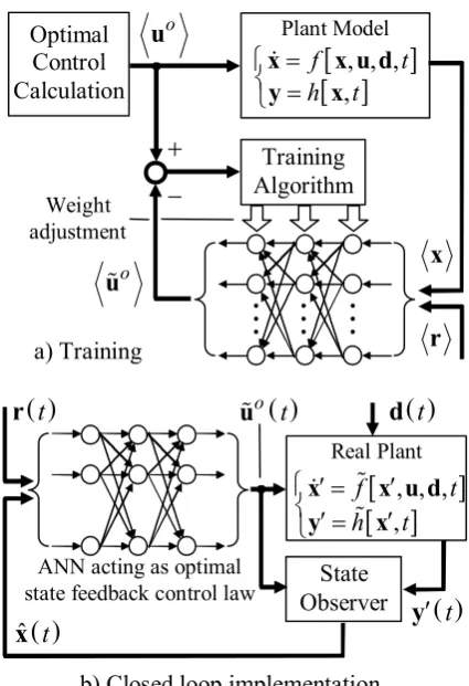
5.2 State Control based on Artificial  Neural Networks: 

Suppose  a  particular  optimal  control  value, 

o 

u  ,  has  been  calculated  off  line  that  should  be applied to the plant given a state value,  x,  and  a  constant  reference  input,  r.  Then,  in  principle, an artificial neural network (ANN)  can be trained to  reproduce an estimate, u %  , o  of u  if  it  is presented with  x  and  ro  . Now  this process could be repeated with the same  ANN  so  that  it  is  capable  of  reproducing  several  different  optimal  control  values 

previously  calculated  off  line  for  different  plant  states  and  reference  inputs  when  presented  with  the  same  plant  states  and  reference inputs. 

Since  digital  processors  operate  in  discrete  time,  the  optimal  control  computational  methods actually yield a set of states,

( )

,

( )

1 , , 

(

1 

)

 

k k k k 

o N 

t t t _-

é ù

= ë û 

x x x K x  (51) 

and a corresponding set of optimal controls,

( )

,

( )

1 , , 

(

1 

)

 

ok ok ok ok 

o N 

t t t _-

é ù

= ë û 

u u u K u  (52) 

at  N  discrete  times,  t t_{0 1}, ,K , t_{N - 1} ,  for  a  constant  reference  input,  r  ,  where  the k superscript,  k,  refers  to  the  particular  reference  input.  Let  the  complete  set  of  results of these off  line  computations over  a  range of  R  different reference inputs be 

1 2 

, ,  R

= 

x x x K x  (53) 

and 

1 2 

, , 

o o o o R

= 

u u u K u  (54) 

Then,  in  principle,  a  suitable  ANN  could  reproduce an estimate,  u % o  , of  uo   , given 

x  and  r =  r r0, 1 ,K , r R .    The  overall  result would be that the ANN could be used  to  directly  close  the  loop  with  an  approximation to control law (50):

(

, 

)

 

o o

= 

u%  G% x r  (55) 

Fig..  2  summarises  the  training  and  implementation stages. 

[image:9.595.71.284.278.589.2]

input  value,  r,  not  included  in  the  original  training  set but lying inside the multidimensional  polygonal  surface  encompassing  the  training  set,  then it should produce a control value, u %  , that is a o  close approximation to the correct optimal control  value, u  . The success of this scheme would, of o  course,  depend  on  the  type  of  ANN  selected  and the number of neurons in the hidden layers.  The  reader  may  refer  to  texts  such  as  (Sunan,  et.  al.,  2004)  or  (Picton,  2000),  to  gain insight into the various types of ANN. 

Fig. 2. Application of ANN for optimal state control. 

6. Conclusions and Recommendations:

 

The  comparison  of  the  two  classical  open  loop  approaches  to  solving  the  optimal  control problem  is  interesting. The dynamic­  programming  method  yielded  one  nonlinear  partial differential equation (15) to be solved 

while applying the maximum­principle to the  same problem yielded two nonlinear ordinary  differential equations (32) and (35). Although  both  techniques  generate  equations  which  require  the  aid  of  digital  computers  for  solution,  the  two  first­order  ordinary  differential  equations  from  the  maximum­  principle  are  considered  easier  to  solve  than  the  nonlinear  partial  differential  equation. In  general,  therefore  Pontryagin’s  method  is  recommended, but Bellman’s  method should  still  be  considered  as  in  particular  cases  it  might prove to be more straightforward.  In order to determine the attainable  closeness  to optimality, it is recommended that the new  scheme depicted in Fig. 2 is  first tested with  very  simple  well  known  cases  for  which  exact closed loop optimal controllers already  exist, such as the double integrator plant. The  next  recommended  step  is  to  test  out  the  scheme  depicted  in  Fig  2  for  the  simple  minimum  energy  control  problem  presented  in section 4. The variation of the closeness to  optimality with the number of training points  and  their  distribution  within  the  operating  envelope of the plant should be investigated. 

7. References:

 

Bellman R.,Dynamic Programming,Princeton  University Press, Princeton, NJ, 1957.  Bellman, R., Dreyfus S. E.,Applied Dynamic Programming,  Princeton University Press, Princeton, NJ, 1962.  Bolttyanskii,  V.  G.,  Gamkrelidze,  R.V.,  Pontryagin, L. S, The Mathematical Theory of  Optimal Processes,I. The Maximum Principle,  Izv., Akad., Nauk, SSR, Ser. Mat. 24, 3, 1960. 

Pearson A. B., “Synthesis of a Minimum Energy  Controller subject to Average Power Constraint”,  Joint Automatic Control Conference Proceedings,  New York, 1962, pp. 19­4­1 to 19­4­6. 

M

M

M

 

a) Training 

b) Closed loop implementation  Plant Model

[

]

[ ]

 

, , ,  , 

f t 

h t

= ì í ₌ î 

x x u d 

y x 

& 

Training  Algorithm  Optimal 

Control  Calculation 

o 

u 

x

+

- 

r 

Weight  adjustment 

Real Plant

[

]

[

]

 

, , ,  , 

f t 

h t

ì ¢= ¢ í

¢= ¢ î 

x x u d 

y x 

% &

%

( )t  

¢  y ( )t  

d 

o 

u % 

State  Observer ( )t  

r o ( )_t  

  u %

( )  ˆ  t  x 

Picton P., Neural Networks, Palgrave, 2000.  Pontryagin  L.  S.,  Optimal  Control  Processes, Usp. Mat. Nauk 14, 3, 1959. 

Optimal  Relay  and  Saturating  Control  System  Synthesis  Ryan,  E.  P.,  Optimal  Relay  and  Saturating  Control  System  Synthesis, P. Peregrinus for the IEE, 1982. 

Shinners,  S.  M.,  Modern  Control  System  Theory and Design, John Wiley & Sons, pp  632­668, 1992.