Perspectives and Advances in
Parameter Estimation of Nonlinear Models
Milena Clarissa Cuellar Sanchez
Supervisor: Professor Leonard A. Smith
Department of Statistics
The London School of Economics and Political Science
University of London
UMI Number: U615661
All rights reserved
INFORMATION TO ALL USERS
The quality of this reproduction is dependent upon the quality of the copy submitted. In the unlikely event that the author did not send a complete manuscript and there are missing pages, these will be noted. Also, if material had to be removed,
a note will indicate the deletion.
Dissertation Publishing
UMI U615661
Published by ProQuest LLC 2014. Copyright in the Dissertation held by the Author. Microform Edition © ProQuest LLC.
All rights reserved. This work is protected against unauthorized copying under Title 17, United States Code.
ProQuest LLC
789 East Eisenhower Parkway P.O. Box 1346
S ta te m e n t o f A u th e n tic ity
I confirm th at this Thesis is all my own work and does not include any work completed by anyone other than myself. I have completed this docu ment in accordance with the Department of Statistics instructions and with in the limits set by the School and the University of London.
Date: O S .0 7
1
Library
Abstract
Nonlinear methodologies to estimate param eters of deterministic nonlinear
models are investigated in the case where experimental observations are avail able and uncertainty sources are present, e.g. model inadequacy, model error
and noise. The problem of param eter estimation is interpreted from a non linear dynamical time series analysis perspective; however deterministic and
probabilistic techniques originated outside the nonlinear deterministic frame work are studied, implemented and discussed.
Conceptually, the Thesis is divided in two parts th a t explore two funda mentally different approaches: (a) Bayesian and (b) Geometrical estimation.
Both approaches attem pt to estimate param eters and model states in the case where the system and the model used to represent it are identical, i.e.
Perfect Model Scenario (PMS), even though the implications of the results obtained are considered for Imperfect Model cases. The performance of the
resulting model param eter estimates in control monitoring and forecasting of
the corresponding system is assessed in an application-oriented fashion and contrasted where possible with system observations, in order to look for a consistent way to combine probabilistic and deterministic approaches. Given
the observations available, combined methodologies enable us to best inter
pret the resulting estimates in a probabilistic framework as well as in the context of a particular application.
The first conceptual part relates to the REMIND project, which is to find
a way to meld advances in nonlinear dynamics with those in Bayesian esti
mation for both mathematical systems and real industrial settings, i.e. for control monitoring the UK’s electricity grid system efficiently. Bayesian in
ference is used to estimate model parameters and model states using Markov Chain Monte Carlo (MCMC) techniques. For the observations of grid fre quency and demand, the operational constraints of the d ata sets are main tained through the estimation process, for example in the situation where the data are provided at rates th at restrict on-line storage and post process
ing. When MCMC is applied to the Logistic Map, curious behaviour of the convergence of the Markov Chain and in the resulting param eter and states
estimates are observed and are suspected to be a consequence of high multi
modality in the resulting posterior, which in tu rn generates estimates with a low dynamical informational content. In the case when the MCMC is applied
to a UK’s grid frequency dynamical model, the technique is implemented in such a way th a t gradually transform from the PMS case into a more realistic
tional data, which fails to provide the information required by the tailor-made
MCMC implementation. In addition, sanity checks are proposed to establish
meaningful convergence of MCMC analyses of tim e series in general.
The second conceptual part explores a new approach to param eter esti
mation in nonlinear modelling, based on the geometric properties of short
term model trajectories, whilst keeping track of the global behaviour of the model. Geometric properties are defined in the context of indistinguishable
states theory. Param eter estimates are found for low dimensional chaotic systems by means of Gradient Descent methods (GD) in the PMS. Some of the advances are made possible by means of improving the balance be tween information extracted from the observations and from the dynamical equations.
As a result of this investigation, it is noted th at, even with perfect knowl edge of system and noise in both models, the uncertainty in the dynamics
cannot be distinguished from the uncertainty in the observations. In ad
dition, the Geometric approach and Bayesian approach of the problem of model param eter and state estimation for nonlinear models in the PMS are
C ontents
1 The Problem 8
1.1 In tro d u c tio n ... 8
1.2 Statem ent of the P r o b l e m ... 12
2 Background 21 2.1 Bayesian Param eter E s tim a tio n ... 23
2.1.1 MCMC T e ch n iq u e s... 29
2.1.2 Simple E x am p le...39
2.2 Maximum Likelihood Param eter E s t i m a t i o n ... 56
2.3 Indistinguishable States ... 58
2.3.1 Gradient Descent A lg o rith m ...63
3.2 Example: Bayesian Inference for the
Logistic Map ... 74
3.2.1 MCMC for the Logistic Map: In P ra c tic e ... 81
3.2.1.1 Full Conditional Distributions: PMS Logistic M a p ... 85
3.2.1.2 Naive Statistical Approach for the Logistic Map 88 3.2.1.3 Using WinBUGS: Chaotic B u g s ... 97
3.2.1.4 MCMC “Tailored” Im p le m e n ta tio n ... 105
3.3 Distinguishing D y n a m ic s...110
3.4 Summary ...133
4 D istilling Inform ation in the Param eter Space 139 4.1 Statistical A p p r o a c h ... 147
4.1.1 Inclusion of Global B e h a v io u r ...161
4.2 Geometric A p p r o a c h ... 167
4.2.1 Search in the Param eter S p a c e ...175
4.2.1.1 Implied Noise Level ... 177
4.2.1.2 Shadowing D istrib u tio n s ...186
4.3 S u m m a r y ... 192
6 Param eter E stim ation from Real Tim e Series: The U K Elec
tricity Grid Case 217
6.1 The Problem ... 225
6.1.1 The Real D a t a ...227
6.2 Grid Frequency Dynamics: Structural Model ...231
6.3 ReMS: Forward S im u latio n ... 240
6.4 PMS E xperim ents... 243
6.4.1 Experiment 1: D a t a ... 246
6.4.1.1 Sub-sampled Frequency and D e m a n d ...247
6.4.1.2 Real operational C o n d itio n s... 248
6.4.2 Experiment 2: Perfect Model ...248
6.4.2.1 Frequency Response F u n c tio n ...249
6.4.2.2 Integration S c h e m e ... 250
6.5 Bayesian param eter Estim ation for the UK’s Grid System . . . 252
6.5.1 MCMC Im p le m e n ta tio n ... 264
6.5.1.1 Likelihood T e r m s ... 269
6.5.1.2 Prior T e rm s ... 272
6.5.1.3 Full Conditional D istrib u tio n s...278
6.5.2 ReMS: MCMC Estimates ...285
6.7 S u m m a r y ... 296
7 Summary and Further Work 301
References 313
Glossary 327
Index 330
List o f Figures 336
A la memoria de mi abuelita Alcira
y dedicada a cada uno de mis abuelos:
a mi abuelito Carlos, el papa de mi mama;
a Mariachi y el abuelo Rafael, los padres de m i papa.
Cada uno ha contribuido con la historia de su vida,
de diferentes maneras y proporciones
a lo que mis padres han sido y son ahora,
y en consequencia lo que yo soy.
Todos han tenido vidas extraordinarias y magicas
que han cultivado en mi curiosidad
y capacidad de seguir siempre adelante
disfrutando y admirando cada momento,
solo mirando atras para reir de lo que ha sido
y mirando hacia adelante con respeto,
A ck n ow led gem en ts
There are many people th a t has been a part of the whole process of my doing a Ph.D.. Thus, I will like to thank them all, going one by one as far as I remember them all, if I do not remember you, be sure th a t as soon as I print the last version I will remember you and I will thank you from my heart.
I would dike to greatly acknowledge Luis, my partner, friend, husband, colleague, and many other things at the same time; without his support and encouragement, at all levels, this story might have been very different. These long four years have been a great adventure for us, where laughter was and continues being the most im portant aspect of it all.
To my family, th a t has been always there for me. Being apart from them has been a great challenge but at the same tim e a confirmation of the strong motivation they had cultivated in me (and all my sisters) to go always forward looking for new challenges in both personal and professional life. I would like to thank my father, Rafael, for his encouragement and support towards my professional development; my mother, Olga, for her inspiring will to go beyond any trouble in life; my aunt Fulvia for her discipline and motivation given to all her nieces and nephews to pursue professional goals; my sisters: Monica Concepcion, Marcela Cristina, M aria Carolina y Mayra Constanza, for all their love and caring for me; and my niece N atalia for her happiness and joy for life.
Many people have taken the place of family members during these more th an four years: my sister-in-law M aria for her support in many practical and logistic aspects of my life in UK; her children Violeta and Fidel for their caring and closeness to me; Nati, my mother-in-law, and Luis’ sisters: Pilar, Teresa, Begona and Alicia; th a t had taken me inside their family and I will appreciate th a t forever. I feel at home with them.
To my friend Alexandra Olaya, for all the times we shared laughing. During this time, we have been reflecting each other p ath in “parallel” worlds. She is my foreing sister.
To Lenny whom has believed in me and has supported me through many moments and situations. I learned many things from him when he has been close or away. He has the spark to influence the life of people around him. I will be always grateful to him.
To my colleagues in LSE, everyone has touched both my personal and pro fessional life and my main reason to thank them is th a t they have showed me the diversity of ways life can be approached: Kevin Judd, Devin Kilminster, Edward Tredger, Sarah Higgings, Antje Weisheimer and Frank Kwasniok. To Liam Clarke I own special thanks. He has the talent to find simple metaphors to explain things and has been a guiding light through the NGT project and the time I spent in CATS. To Jochen Brocker for his friendship and useful and sharp comments in many informal discussions, and to Du Hailiang for his natural brightness and hard work during joint work and also th a t I learned how to properly fry spring rolls.
To the NGT team th a t supported us through the REMIND project and the Smith Institute, specially to Melvin Brown, Hai Bin Wan, and Ahmad Chebbo. I will also like to thank: Imelda Noble, Esther Heyhoe, Lyn Grove, Inesh, Emma and Paul, Tina, Effie, Claudio Zappia, Monica and Duncan McLeod.
This project was financially supported by a grant awarded to LSE by the National Grid Transco, Pic. My scholarship was enmarked in the EPSRC, REMIND project managed by the Smith Institute for Industrial M athematics and System Engineering. Additional financial support was awarded to me annually by the Department of Statistics at LSE, throught G raduate LSE Scholarships. W ithout this financial support all this adventure could not have been possible.
C hapter 1
T h e P rob lem
1.1
Introduction
The behaviour of natural and artificial systems has captured the attention
of humans since the beginning of mankind. Every moment of every day, rationalisation of surrounding phenomena is performed.
Observations are constantly obtained and used in order to characterise
and attem p t to control the surrounding reality. Sets of rules are assigned
to represent this reality with the aim of reproducing the observed phenom
ena. These sets of rules are the models th a t represent reality and differ from subject to subject depending on many different aspects such as current cir
secure and malleable—or it feels so at any rate. Although no model can
change reality directly, such models help understand the world.
The information obtained from observations is incomplete and is fre quently corrupted. Furthermore, it is normally impossible to acquire all
the relevant information needed to assign a consistent set of rules. As a
consequence, the model is just an approximation of reality. Models used to represent reality are sometimes mistakenly thought of as reality itself, given
the success of the model. Even when the chosen model does not provide a very accurate representation of reality, it is taken as reality itself.
Modelling reality plays a key role in the scientific m ethod and in the applications of its laws and developments towards particular applications.
In this very restricted context, reality is the system where the phenomena of interest happens, and observations are quantities th a t can be measured, i.e. quantities with units. Observations contain information on the system
and are used to formulate a model or to refine a previously formulated one.
Models are mathematical structures th a t formally described the system. In the process of gathering all relevant information about a system, many
obstacles are encountered. For example, storage capacity is finite, measure
ments cannot be performed in continuous time, measurement devices have finite resolution, not all relevant variables can be observed and there are
formation available is uncertain. In addition, given th at only observations
are available, discriminating the nature of a system, i.e. stochastic or deter
ministic, is impossible [64]. Therefore an a priori choice of a stochastic or a deterministic model is arbitrary.
Although uncertainty makes the view of reality fuzzy, it also can be used to extract useful information. In more optimistic terms, uncertainty in the
observations and in the model chosen to represent the system may highlight the relative ability of a model to represent the system in terms of forecasting
or control monitoring.
This Thesis focuses on the situation where model param eter values are to be found once a model has been formulated to represent a system of interest. Param eter estimation is a fundamental problem in both stochastic
and deterministic frameworks although it is approached in different ways. This work follows the idea th a t there is no “proper methodology” for param eter estim ation when the only source of information is a time series.
Furthermore, it considers two model choices to be used to represent the
dynamical system: (1) separable dynamical models th a t are deterministic but contain a separable stochastic component referred to throughout this Thesis
as measurement noise, and (2) stochastic dynamical models th a t contain
of the two model choices is justifiable when formulated towards coping with
uncertainty sources in the system. Given a particular system, validation of model choice and definition of “good” estimates are made from out of sample
performance.
The use of dynamical models th a t can be either stochastic or determin istic leads to approaches to solve the problem of param eter estimation th a t
meld methodologies from statistical and nonlinear times series analysis frame works.
In this Thesis, the problem of param eter estimation is interpreted from a non-linear time series analysis perspective; however, techniques originated outside the nonlinear deterministic framework are studied, implemented and discussed for dynamical systems.
This Thesis is structured as follows. C hapter 1 formulates the problem in
simple terms. Chapter 2 introduces the techniques used at different stages
in the research for particular applications and provides an overview of what is new in this Thesis.
C hapter 3 uses Bayesian methodologies of param eter estimation to esti m ate param eters for the Logistic map [24]. The Chapter presents a correct
formulation of the problem of param eter estim ation in Bayesian terms and
implements a tailored MCMC routine for this case [23].
distinguishable state theory [54, 55] and ensemble construction to search for
param eter estimates in nonlinear models.
Chapter 5 contrasts system state estimates obtained by two different ap proaches, Bayesian and dynamical. It provides interesting results which lead
to an extensive plan of further work.
C hapter 6 describes the attem pts and results to estim ate param eters for
a simple model of electricity grid frequency dynamics [20] using Bayesian methodologies and real experimental d ata [22].
Finally, Chapter 7 lists the new results and general outcomes of this work,
highlighting further research in this area.
1.2
S tatem ent o f th e P roblem
Let S' be a time series of observations of a system ’s tem poral evolution. The
tem poral evolution of the system is given by the map, f { x t \ 0) : Rm — ► R m,
where at time t, the system state is given by
x t = f ( x t-1; 0 ), (1.1)
x t £ R m are the system states at time t £ Z and 0 £ R^ is the fixed value for the true param eter vector of the system.
sys-tern’s temporal evolution and the model chosen to represent it. The possible
scenarios are:
1. The Perfect Model Scenario (PMS):
The system and the model share the same m athem atical structure.
Therefore, x t = x t for all t; thus f = f . Given th a t the system’s
temporal evolution is given by / for a fixed value of the param eter vector 0, the model chosen to represent the system is chosen from the model class / ( • ; 9).
In the special case where the tem poral evolution of the system states, x tl is modelled by the deterministic map, f = f ( x t \0) : Rn — ► R n,
x t+i = (1.2)
where x t for all t are the model states and 0 G R^ is the model param
eter vector. The map in equation (1.2) can be w ritten in term s of an unknown initial condition xq by the t—fold composition of / as
x t+ i = / * ( z o ; 0 ) . (1.3)
At time t, it is assumed th a t all components of x t are observed, i.e.
n = m, and the d ata point st e R 771 is recorded. In other words, the sampling rate is constant. The length of the d ata set S is N G N, and
Given th a t each observation is subject to noise, the measurement noise
component is
st = x t + r]u (1.4)
where r)t G Mm and rjt ~ IID (0 ,a ^ ), an independent and identically
distributed random variable with known variance a
Notice th a t in some cases, the system under observation is physically under the influence of internal random fluctuations. Therefore the sys tem states, x t, are randomly perturbed by dynamical noise. If the unknown initial true state of the system is xq, the additive dynamical
noise is mathematically represented as
%t=1 = f ( x 0 + 6o;0),
%2
=
/(£i + ^i;0),
x t = f ( x t- i + 6 t- u 0 ) ,
x t+i = f { x t + 6t ]0). (1.5)
where 8t G Rm is a random variable w ith unknown mean and variance,
The perfect model scenario case can be dressed in two ways:
noise, the PMS is a separable dynamical model given by equations
(1.2) and (1.4), explicitly,
s t - f t{ x o \ 0 ) + r)u (1.6)
for t > 0. Note th a t in this case, the sequence of states, {^t}t>o, is indeed a trajectory of the system.
(2) The observations of the system (1.1) contain both additive noise
components, the PMS is a stochastic dynamical model given by equa tions (1.2) to (1.5). Explicitly,
st = x t + rjt, (1.7)
where x t = f ( x t-1 + 5t- i) thus
s t = / ( / ( • • • /( /( ® o + ^o) + <5>i) H 5 t ~2) + f i t -1) +f7tj (1*8)
' v '
t tim es
for St ~ IID(0,(Tfi). Therefore, the sequence of states, {£t}t>o, is no longer a trajectory of the system
The admission of the presence of dynamical noise in the observations
may sometimes be seen as a “shadow” in low dimensions of higher
system states during the experimental process of gathering system ob servations. The effects on the dynamics from the presence of both noise
types are studied in detail in [11] for chaotic systems.
2. The Imperfect Model Scenario (IMS):
The system is approximately represented by the model. Therefore,
f — f and Xt 7^ Xt- Perfect models are not available in cases where d ata comes from physical systems ([55] and references therein). The
“Laws of Physics” are only a useful approximation of the system un der well defined conditions [15]. Model inadequacy arises when the model chosen to represent the system is structurally incorrect, is phe
nomenological not derived from any physical principles, does not in clude unknown and not observed dynamical components of the system, involves coarse measured variables or variables representing averages,
among other factors.
The only information available about the system states is provided by the observations recorded at time t. Given th a t the system / is
represented by an imperfect model, of the same dimension, / : Rm —►
Rm, it is assumed the observation are st G Rm, i.e. live in the same space Rm, and are recorded at a constant rate, with no loss of generality.
times the system trajectory is observed.
The measurement noise is mathematically represented by
st = x t + T]t , (1.9)
for rjt ~ I I D (0, <jf) and the Xt s, t > 0, are the imperfect model states. Comparing equation (1.4) for the PMS and the equation above shows
th a t the difference is th a t in the IMS, systems states are not available, only imperfect model states.
In this Thesis, model inadequacy or impersection is represented by an artificial dynamical noise component in the model, w ritten as
xt+i = f { x t \ 0) + 5t+1, (1.10)
for St G Mm, St ~ IID (0,(jfi) where erf is uknown. 5t is called arti
ficial dynamical noise (c.t. equation (1.5)), and by no means, it does represent any random perturbation physically happening in the system.
In this context, dynamical noise is then interpreted as model error
rather th an as a property of the observations.
3. The Real Model Scenario (ReMS):
In this case, the system is complex; / , does not exist and there is no
of the system dynamics; Observations are noisy and finite, and all
available models are a simplification of the current state of the system.
The ReMS is a special case of the IMS, and it is known th a t the model used to represent the system is an ignored-subspace model [55] since it
does not include an unknown and unobserved dynamical component of
the system, and involves coarse measured variables or variables repre senting averages. This scenario is exemplified in Chapter 6 for the grid frequency dynamics.
Two different approaches are used throughout this Thesis in the attem pt to estimate model param eter estimation from observations:
A. The Naive Realistic Approach (NRA):
Given a system in any of the scenarios described in parts 1 to 3, the model is assumed to be a perfect model describing the system. Differ
ences between system and model are neglected and model error is not taken into account.
B. The Naive Statistical Approach (NSA):
Given a system in the PMS, the model is assumed to be stochastic even though the perfect model is known to be a nonlinear deterministic model. Although the stochastic model is inadequate to describ the
cope better with some uncertainty sources in a statistical framework.
The dangers of assuming a model class as perfect ignoring the natural
difference between system and model are clearly posed by Chatfield [19] in
Chapter 3 and Chapter 13, respectively:
"... there is a real danger that the analyst will try many dif ferent models, pick the one that appears to fit best ... but then make predictions as if certain that the best-fit model is the true model. ”
“When a model is selected using the data, rather than being specified a priori, the analyst needs to remember that (1) the true model may not have been selected, (2) the model may be changing through time or (3) there may not be a ‘tru e’ model anyway. It is indeed strange that we often implicitly admit that there is un certainty about the underlying model by searching fo r a ‘best-fit’ model, but then ignore this uncertainty when making predictions. In fact it can readily be shown that, when the same data are used to formulate and fit a model, as is typically the case in time-series analysis, then least squares theory does not apply. Parameter es timates will typically be biased, often quite substantially. In other words, the properties of an estimator may depend, not only on the selected model but also on the sesection process. ”
Chapter 3 of this Thesis explores issues related to param eter estimation in the PMS as defined in part 1 and also it uses intentionally the NSA to ob
tain estimates of parameters and non-observed variables in order to compare with earlier results shown in [70]. Chapter 4 estimates model param eters for
chaotic maps in the PMS from observations th a t contain only measurement
noise as formulated in [68]. A ttem pts to implement methodologies of pa ram eter estimation in the IMS for the special case of the real model scenario
to formulate a dynamical model. Once the model is formulated, the NSA is
used to obtained param eter estimates from real d ata sets, assuming as PMS the imperfect model class formulated for the grid frequency dynamics.
The final solution to all parts of the problem, in particular part 2, i.e. the
imperfect model scenario, where even the existence of “optim al” param eter values is doubtful, is beyond of the scope of this Thesis.
C hapter 2
B ackground
Assume th a t a time series of observations of the system of interest is available. The features of the system’s tem poral evolution are to be used to characterise the system for purposes of forecasting and control monitoring tasks. Looking at the tim e series of interest, the system under study is represented as a
m athem atical structure or model. Once this model-system relation is set,
the problem of model param eter estimation from time series is understood as a model fitting problem. Uncertainty is present in the observations and in
the model chosen to be the representation of the system. Methodologies used to solve this problem should include considerations of uncertainty sources to
increase the reliability of the resulting estimates.
the methods used at every stage of this investigation on how to find param eter estimates for nonlinear models. The Chapter is a list of recipes of the relevant methods for param eter estimation, and discussion of the issues related to the
problem of interest is found in the main Chapters of this work.
A statistical approach to this problem is called inference or model eval
uation. In th a t context, inference is the process of updating probabilities
of outcomes based upon the relationships in the model and the evidence known about the situation at hand [9]. This Chapter presents the statis tical methodologies from the Bayesian and the Frequentist perspectives in
section 2.1 and 2.2 respectively.
Traditionally, in the nonlinear dynamical perspective, uncertainty in the
observations given by noise presence is accounted for by noise reduction meth ods [58, 16, 36, 26, 92] whilst methods to account for uncertainty in the model are still in development and subject to continuous progress [19, 87, 75, 54, 55,
51]. section 2.3 presents the way indistinguishable states are found for the
chaotic Logistic map [67] by means of the gradient descent (GD) algorithm following the work of Judd and Smith [54, 55].
In general terms, there is no m ethod which could be labelled as a “proper”
identify the nature of all uncertainty sources. In most cases, there is a trade offs between the relevant information obtained while reducing uncertainty on the “uncertainty” of the nature of the uncertainty sources themselves. A suc
cessful methodology is one th a t balances such trade-off for a given scenario
in the context of a particular application.
2.1
B ayesian Param eter E stim ation
Bayesian inference is a statistical approach to estim ate and predict a be
haviour of interest [95, 70, 12]. In this framework, probabilities are inter preted neither as frequencies, proportions nor likely events. Instead, this ap proach can be seen as a way to formally model a system in terms of probabil ity distributions. These probability distributions combine “common-sense”
knowledge and observational evidence [29].
Prom the Bayesian point of view, there is no fundamental distinction
between variables and param eters in the model used to describe the situation of interest. In the first instance, param eter and model variables are both
naively assumed to be random variables, if the model is a dynamical nonlinear system.
A distinction is made, however between observable and non-observable
can be measured in the experimental process of observation, i.e. it can be
replaced by d ata values. Often the non-observable random variables are
called parameters, regardless of being model parameters or model variables. In order to translate the statem ent of the param eter estimation problem
for a dynamical system to the Bayesian framework, model variables, param
eters and observations are classified either as observables or non-observables. The notation defined in Chapter 1 is going to be stretched in the Bayesian
framework in a way th a t all observables are collected in S whilst all non observables in the Bayesian param eter vector 0.
The statem ent of the problem in Chapter 1, section 1.2, provides a defi nition of the system dynamics of interest in equation (1.1), a d a ta set S of noisy observations (see equation (1.4)) and a model to represent the system
dynamics given by equation (1.2).
Prom this statem ent of the problem and the principles of Bayesian in
ference, classification as observables and non-observables is made as follows, and it is independent of the scenario the model is placed.
• Observables, S:
constrained to the known values of zero and cr^, respectively. Therefore,
the observables in S are all observations { st} £ i and the two known param eters of the noise process, producing a set of observables with
N + 2 elements.
• Non-observables, 0:
After finding the observables contained in S, the rest of model param eters and variables are all included in the Bayesian param eter vector
0. The param eter vector includes the model states {zt}£Li, the ^ ~ tial condition Xq and the I model parameters in f { x t \ •), making 0 of
dimension N + 1 + 1.
Note th a t for particular examples, the param eter vector 0 will also in
clude hyper-parameters [95], parameters of the random process associated to a component of 0, which in tu rn will increase the dimension of the Bayesian param eter vector. Choice of hyper-parameters related to components of 0 is
drawn from relevant background information on the system to be modelled, and it is denoted as I, following notation in [83].
Bayesian statistical inference requires setting up a joint probability distri
bution, p(S, 0\I), of all random variables [95]. The joint probability density function (PDF) can be decomposed into the product
where p{0\I) is known as the prior distribution of all non-observables and
p (S \0 ,1 ) is called the Likelihood: a conditional PD F of all observables given
the non-observables. As noted before, the prior contains all the information about param eters which is obtained by having knowledge about the situation
before observing a d ata set S. The information coming from the experiment
is contained in the Likelihood.
The prior and the Likelihood are updated via Bayes’ theorem [4] to a
probability distribution of the parameters, given a realisation of the d ata set 5, as follows:
f0 |c n = p ( s \ 0 J ) Pm ,2 2 ,
P{ 1 ’ ] fp ( S \O ,I ) p ( 0 \I ) < i0 { - ] where p ( 0 |5 ,1) is called the posterior probability distribution. The posterior is the distribution th a t contains all the samples from the prior th a t best resemble the d ata given the d ata set S [95], and the relevant background
information I. The background information I is also referred to as prior information.
The denominator in equation (2.2) is a normalisation constant with re
spect to 0. This distribution is known as the marginal distribution, m (S \I), given by
m ( S \I ) =
J
p (S \0 ,I)p (O \I)& 0 (2.3)each of the PD F involved in equation (2.2) is made to stress the fact th a t once
the background information is different, the functional form of the posterior is changed.
In practice, a major technical difficulty in the implementation of Bayesian
methods is the high dimensional integration involved in m ( S \I) and in the calculation of any expected value of the posterior distribution. The numerical
implementation of Bayesian methods involves sampling algorithms th at draw realisations from the posterior distribution. The m ajority of these algorithms
are formulated in terms of non-normalised distributions.
In these terms, it is more convenient to write equation (2.2) as
Once a realisation of S = S' is obtained, equation (2.5) is evaluated on S so th a t the posterior distribution p ( 0 \S ,I ) is a function of 0 only. Thus
the posterior distribution p(0\S, I) is denoted by 7Ts{0\I)- This new notation
for the posterior emphasises the fact th a t the posterior distribution (2.5) is
different for a different realisation of S and what is considered in a particular case as relevant background information I. The PD F, t t s { 0 \ I ) is known as
the full joint posterior distribution.
Formally, let S = {sj£Lx be the set of observations of the system of in p ( 0 \S ,I ) oc p ( S \ 0 , I ) p ( 0 \ I ) (2.4)
terest, where st G R m and TV G Z is the length of d ata available. Prom (2.5)
it follows th a t
TTS (0\I) = p ( 0 \ S = { s t } l 1,I ) , (2.6)
is only a function of the param eter vector 0 and the prior information /.
The joint posterior distribution 7ts(@, -0 is the object of interest in the
Bayesian framework since, in principle, any inference of any param eter in the model could be made from the knowledge of n s { 0 \ I ) . In general, inference on 0 translates into the calculation of expected values of an arbitrary function of 6, g(0). The expectation of g{0) is defined by
E«,i W ) \ =
J
9(8) ttsW ) M - (2-7)For future reference, lets introduce some detailed notation for the compo nents of the param eter vector 0. Let 6,i G be the ith component of 0 for 1 < k < i and i = 1, . . . , £, and let 0 be all components of 0 excluding the
ith component 0.j. In general, 0* is not scalar, but for simplicity it is assumed
to be scalar thus 0.* G R Vi, with no loss of generality. For example, in this notation and for g($) — 0 equation (2.7) is w ritten as
EvAe.il
= /
B.i *s(0\I)d0
(2.8)
The calculation of such expected values as equation (2.7) involves at
least two high dimensional integrals, one to obtain the marginal distribu tion m ( S \I) and one to project g(0) onto the measure induced by the full
posterior irs{0\I). Such calculation could not be performed analytically and it becomes one of the main practical difficulties when making inference from
a posterior.
In order to address this analytical intractability of the Bayesian formula tion, numerical integration of (2.7) is carried out by a Monte Carlo approx imation. This approximation involves getting random samples of t t s ( 0 \ I )
by suitable sampling algorithms. In particular, samples are taken to be the states of a suitably constructed Markov chain such th a t t t s ( 0 \ I ) is its station ary distribution. The numerical implementation of Bayesian methods using realisations of Markov chains as samples drawn from the full joint posterior
distribution (2.6) and Monte Carlo integration to calculate expected values (2.7) are known as Markov Chain Monte Carlo methods, or MCMC in short.
2.1.1
M C M C Techniques
Monte Carlo integration.calculates the expectation E Vtj[-] in (2.7) by drawing
\
samples are used to evaluate the expectation defined in (2.7) as follows
(2.9)
The set of posterior samples for the param eter vector 0 is denoted by
proportions. Sufficient independence can be understood to mean th a t sam ples of each of the components 0 * of 0 are independent from each other i.e.
p(Q.i,6.i') ~ p(6.i) x p(9.i'),Vi 7^ ir- Now, sufficient independency is achieved by constructing a Markov chain such th a t tts{ 0 \ I ) is its stationary distribu tion.
Under precise regularity conditions (see [29] and references therein) a Markov chain is constructed such th a t when T —> oo, the following asymp totic results are reached with probability one.
As such, the averages of chain values are equivalent to estimates of pa rameters in the limiting distribution 7r. For detailed discussion of this point { 0 ^ \ j — 1» - .,7 } and can be generated by any process which draws “suffi
ciently” independent samples throughout the support of 7 T s ( - | / ) in the correct
lim 0 ^ — ►0 ~ 7Ts{0\I)
T->oo (2.10)
and
(2.11)
MCMC is an iterative process in which samples of the components of 0
are obtained from the states of a suitable Markov chain. Each state of the
chain is a complete sample of the param eter vector 0 at a given iteration j. Most of the effort is put in the generation of suitable chain states since
inference is reduced to calculate geometric averages.
A suitable Markov chain is one whose transition probability, p ( 0 ^ ^ \ 0 ^ \ /) , converges to the joint posterior tts{ 0 \ I ) in the limit T —*■ oo[66]. The tra n sition probability is the conditional probability th a t the current state of the chain 0 ^ becomes the state 0 ^ +1\ This probability is also known as the
transition kernel of the chain, and it is denoted by K ( 0 ^ +1^ \0 ^ ) .
Typically, the Markov chain takes values in R£, since 0 £ R*, and a Markov chain is constructed using the algorithm developed by Hastings [40],
which is a generalisation of the method developed by Metropolis et al. in 1953 [69], and is known as the Metropolis-Hastings (MH) algorithm [40, 69,
30].
The MH algorithm generates a sequence { 0 ^ } J =i as follows:
Set i n i t i a l c o n d itio n s : $ U = ° )
Loop ( j = 1, . . . , T ) {
Sample a candidate s ta te j + 1 : Y ,( . ie » )
Sample a uniform random variab le: U rsj U(0,1)
I f : U < a { p t i \ Y ) then: 0 U + V = Y
otherw ise: = @( j )
The algorithm proceeds at each time j by choosing the next state of the
chain 0 ^ +1^ by first sampling a candidate state Y from a proposal distribu
tion q ( '\ 0 ^ ) which depends on the current state 0^t+1\ The candidate Y is accepted w ith a probability of acceptance given by
a { 0 ^ \ Y ) = min ;r ( y |/ ) 9(0 “ |y )
^■(©“ IJ) q { Y|0O)) (2.12) The proposal distribution <?(-|-) could be in any functional form and the stationary distribution of the chain is 7 r ( - |I) provided th a t the transition
equation in (2.13) constrains the rates of moves through states in detail for
see [9, 29, 95].
It is often more convenient and efficient, from the com putational point
of view, to divide 0 in components {0 1, 0.2, . . . , 0.*,..., and then update these components one at a time. It is not necessary for each component to
be scalar. W hen the param eter vector is divided into components, the up dating process used for constructing the appropriate Markov chain is known kernel for the Metropolis-Hastings algorithm satisfies the detailed balance
equation
ir(x) K ( x , y ) = ir{y) K ( y , x ) (2.13)
when the chain moves from x = 0 ^ to y — 0 ^ +1\ The detailed balance
every possible pair of states. Therefore, once 0® ~ t t s ( 0 \ I ) is obtained, it
as the single-component Metropolis-Hastings algorithm and was the original
structure proposed by Metropolis [69].
At each time step, the algorithm updates each of the I components of 9
using the Metropolis-Hastings algorithm. In the ]th iteration, the state of the
chain is updated one by one for each of the I components of 9. Iteration j
updates O^p for i = 1, . . . ,£ choosing Yti from q i(Y i\9 ^\ 0^ ) as a candidate for the updated value 0 ^ +1^ i.e. the 1th component of the next state in the
chain. Explicitly, the term is
0.-1 = ( ^ '+1), • • • - 0.¥-i \ 0 % , Of ) . (2.14)
Following (2.12), the candidate is accepted with probability
a ( ^ i \ 0.-i> Y.i) = min S 1
where ^ ( 0 ^ 1 0 ^ , I) are the full conditional distributions for i — 1, . . . , A
If Y i is accepted then 0^'+1^ = Yi, otherwise 0^+1^ = and the chain does not move. Note th a t no other component of 6 ^ is changed in step j.
For clarity, the definition of the full conditional distributions is presented later in this section.
By analogy with the description of the MH algorithm, the general struc
Set i n i t i a l cond itions: 0^ °) Loop ( j = {
Set coordinate ite r a to r i = 1
Loop (z = 1, . . . , £) {
Sample a candidate s ta te j + 1: Xi ~ gi(Y]i|0^, 0 ^ ) Sample a uniform random v a ria b le: U U ( 0,1)
I f: U then: 0<f+1) = Y t
o th erw ise: <^+1> = Increment z }
Increment j }.
Note that 0 ^ mixes the values of the components previously already
updated in the current iteration j (see equation (2.14)) and components
updated in the previous iteration j — 1 when 1 < i < i — 1.
Synoptically, given an arbitrary set of starting values 0 ^ , . . . , 0 ^ the first
iteration of the updating process looks as follows:
sim u la te 0 ^ ~ ^(^ i| • • • i -0
sim u la te 0 ^ ~ tt(0.2| . . . , 0 ^ , I )
sim u la te 0(il) ~ 7r(0.i| 0(i }, . . . , 0 ^ 1 ,0(° j i , . • •, 0(° \ I )
• sim u la te 0 ^ ~ 7r(0.^| 0 ^ , . . . , 0 ^ , 7 )
and yields a chain with states 0 ® = ( 0 ? \ . . . , O ^ f ) after j cycles. Con
sequently, if all the full conditional distributions are available, all that is
The full conditional distribution of 0® under 7r(-, I) is defined as
7TS(0|/)
f * s ( 0 \ i ) deA (2.16) Note th a t the normalisation constant in (2.16) is independent of 0j, since from equation (2.6) it is clear th a t the posterior distribution is proportional
to the joint PD F of all observables and non-observables in the model.
In other words, the full conditional distribution of 0*, given the values of the other components 0. corresponds to those terms of n s(0 \I) in which 0A appears explicitly. This feature makes full conditional distributions straight forward to calculate. The process becomes even more straightforward when a conjugate functional form can be easily identified i.e. the full conditional
distribution is in a closed form.
Let T be a family of probability distribution functions f ( x \0 ) (indexed
by
9
) . A class T* of prior distributions /* is a conjugate family for T if theposterior distribution is in the class J7* for all / £ J7, all priors f* £ J7*, and
all x £ X [17, 29]. When this happens, the functional form of the distribution is said to be in a closed form. This class is closed under product, therefore if
f £ J7, the product / • /* £ J7*.
For example, if the Likelihood distribution belongs to the same conjugate
conjugate family. The role of conjugate families of distributions in the prac
tical implementation of the MCMC methodology is very im portant and will
be clearly visible in the example presented later in section 2.1.2 and in the
applications of Bayesian perspectives for the Logistic map in Chapter 3 and
for National Grid dynamics in Chapter 6.
One of the most im portant issues surrounding the implementation of MCMC techniques is the choice of the proposal distribution g(-)[95, 91, 61,
80]. For com putational efficiency, q(-) should be chosen so as to be easily eval uated and sampled from, and with associated high probability of acceptance given by equation (2.12).
A common way to choose the proposal distribution q is the process called Gibbs sampler [32, 30]. The Gibbs sampler is a special case of the single
component MH algorithm, taking as the proposal distribution for the ith component of 0 its corresponding full conditional as defined in (2.16). The
candidate for the next step of the chain is drawn from the full conditional. Therefore the MCMC with the Gibbs sampler is
qi ( Y M i,0 .- i) = 7r(Yi \e.-uI)- (2-18)
Substituting equation (2.18) into equation (2.12) gives
a ( 6 ^ , e % Y . i) = 1, (2.19)
chain.
Having chosen the proposal distribution, the next step is to find out how
the generated Markov chain is converging towards a stationary distribution,
tts{ 0 \ I ) . This problem is known as chain m ix in gand is directly related to the mix values of past and present updates of components 0. Depending on the relation between the proposal distribution q = 7r(* |-) and the full posterior
7rs(-|/), the mixing can happen at different rates. The slower the mixing of the chain, the larger the number of iterations needed to achieve convergency.
For the m ajority of applications, the complexity of the models makes it impossible to calculate analytically the rate of convergence of a particular transition kernel towards the stationary distribution, and it is therefore nec
essary to develop numerical tools to check chain convergence (for a review of these tests see [13]).
To monitor convergence where only one realisation of the chain is avail
able, the output of the Monte Carlo calculation using the posterior samples
from the MH algorithm iteration are plotted and then the number of itera tions of the algorithm when the mixing appears to be achieved is chosen by
eye [95]. W hen parallel runs are available leading to several realisations of
the same chain, the Gelman and Rubin (GR) statistic [31] can be used to assess convergency.
r + 1 , T } contains all T — r — 1 samples from the full posterior ns(0\I).
Thus the estim ator in equation (2.9) is given by
E v A g m « Y 9(0(i)y (2.20)
j= T+ 1
In practice, r should be large enough to obtain consistent estimates. The
size of t is limited by computational resources. Evaluations of the full con
ditional distributions make the numerical implementation costly in terms of running tim e and computational resources, which grow as the complexity of the model increases.
Note th a t the conditioning of the full conditional distributions changes at each iteration (since changes), each full conditional distribution 7Ti(-|0 ^ , I)
being used only once per iteration j and for each component t. Generating random samples for such distributions is, in general, time consuming, even more so when analytical reduction to a closed form for the full conditional
distribution is not possible.
W hen the full conditional distribution is in a closed form, standard al
gorithms should be used to generate random samples. W hen this is not the case, the Accept/Reject Algorithm is used for sampling from a general density fy (y )- This algorithm is presented in [17] as the theorem 3.2.1 in section 3.2.1.4.
sim-pie example presented in Chapter 5 of [95]. The simple structure of this
simple example gives insight on the implementation of the single-component
Metropolis-Hastings algorithm, as well as on the definition, calculation and properties of the full conditional distributions, including the convergence of
the transition kernel of the chain to the joint posterior distribution 7Ts{0\I).
2.1.2
Sim ple E xam ple
Assume there is access to a data set of observations corresponding to reali sations of a random variable Y . In order to infer any moment of Y , requires setting up a probability model to represent it. Let y = { y i,..,2/iv} be N realisations of a random variable Y . Based on I, the background expert knowledge of the process associated with Y , and before any realisation of
the process is observed, the yt *s are chosen to be normally distributed with unknown mean fi and variance <r2
yt ~ £ = 1 , . . . , TV. (2.21)
where are conditionally independent given f i and a 2.
For unknown parameters, no information is available, so the following nori-informative priors are set reflecting / ,
/i ~ ^ ( 0 , 1 ) , (2.22)
where independency between /x and cr2 is assumed and Qa(a, (3) is the generic
notation for a Gamma distribution with mean a / (3 and variance ol/ 0 1 . Prom
(2.23) is clear th a t o2 follows an Inverted Gamma distribution.
Equations (2.21) to (2.23) form a two-parameter Bayesian model. This
model consists of one observable y and two non-observables /x and r . Fol
lowing the notation introduced in last section, the param eter vector is 0 =
2) =
From equations (2.4) and (2.5), the joint distribution of ?/, /x, and r is
given by
N
p ( y, /x, a2\/ ) = Y I P{yt\v, o 2,1) P W ) p( ° 2\I)- (2-24)
t= 1
Substituting equations (2.21) to (2.23) into (2.24),
p { y , p ,a 2) = N
t = 1
N
n
t=i 1
\p2/KO" exp
x AT(0,1) x g a (2 .0 1 ,l),
r (:V t - P ) 2
2a 2 x
- H 2/2 x
r ( 2.oi)(72
- 1/a2 (2.25)
is obtained.
If more relevant information about 0 were available, equation (2.25) had
looked different since the different prior choices. The background information is translated into the priors and Likelihood terms by “relevant” probability
func-tional form of the posterior is written, the explicit notation of the dependency
of equation (2.24) on I is dropped for clarity.
Once the d a ta set S = {ytjtLi is observed, (2.25) is evaluated on the realisation of Y and from equation (2.6) it follows th a t the functional form
of the joint posterior distribution tts{ 9 ) is proportional to #+ iN
irs {0) oc ( — ] exp a 2
As pointed out earlier, to construct the full conditional distribution asso ciated with the param eter 0 * one only needs to pick out the terms in (2.26), where 0 * appears.
Choosing the correspondingly appropriate terms in (2.26), for this two- param eter Bayesian model the full conditional distribution for the mean pa
ram eter is
7r(^|<72) oc e x p j ~ 2 ^ 2 ~ ^ ) 2 “ j ’ ( 2 -2 7 )
whilst for the variance param eter is
7r(<T2|/i) oc ( —r ) exp £ + i
(2.28)
Rewriting equations (2.27) and (2.28), it is easily found th a t the full con
Gamma distributions respectively. These full conditionals are then given by
Note th a t the prior distributions are in the conjugate family of the Like lihood p (y|/x, a 2) in (2.21), and therefore the full conditionals are reduced to a closed form. According to (2.18) the proposal distributions, g, are chosen
as the full conditionals (2.29) and (2.30)..
To generate the first state of the Markov chain given an arbitrary initial
using standard sampling algorithms for Normal and Gamma densities. Af-(2.29)
and
(2.30)
condition 0^ )
simulate r\j
simulate ~ (2.31)
ter T iterations of both simulations in (2.31), a Markov chain {0}J=1 =
tions in (2.31) the single-component MH algorithm described earlier is easily-
implemented.
Three parallel runs of the single-component MH algorithm using the
Gibbs sampler were performed for T = 1.1 x 10⁵ iterations. A set of N=100
observations, randomly distributed as
2* ~ V ( / i , a 2) (2.32)
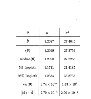
for t = 1 , . . . , 100 and true param eter values 0 = a 2) = (1.2029,27.4045) were observed. Each run generates a Markov chain for the param eter vector
0 — (^.i?
0.2)-Once the chain is obtained, the convergency and mixing have to be as sessed by choosing the burn-in time r where the samples drawn from the full posterior distribution are to be considered as samples of the posterior.
Typically, convergency is physically assessed by plotting the output of a Monte Carlo approximation of any summary statistic, taking the Markov
chain states obtained as samples, when only one chain is available. Plotting
the Monte Carlo approximation of a summary statistic is the simplest way
to check for convergence and mixing, i.e. the param eter space is explored with the support of the full posterior.
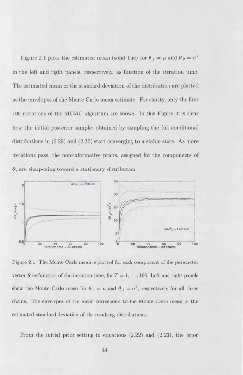
Figure 2.1 plots the estimated mean (solid line) for 6A = ^ and 6,2 = cr2 in the left and right panels, respectively, as function of the iteration time. The estimated mean ± the standard deviation of the distribution are plotted as the envelopes of the Monte Carlo mean estimate. For clarity, only the first 100 iterations of the MCMC algorithm are shown. In this Figure it is clear how the initial posterior samples obtained by sampling the full conditional distributions in (2.29) and (2.30) start converging to a stable state. As more iterations pass, the non-informative priors, assigned for the components of 6, are sharpening toward a stationary distribution.
A v ii A CM ® V - 6 40
Iteration tim e - All cha in s 100
20 60
All cha in s
var(n)T = 3.7 8 8 e-0 4
A ± V II A ® V 0.5,
20 40 60 100
Iteration tim e - All chains
80
Figure 2.1: The Monte Carlo mean is plotted for each component of the parameter vector 0 as function of the iteration time, for T = 1,..., 100. Left and right panels show the Monte Carlo mean for 6 and 0 i = cr2, respectively for all three chains. The envelopes of the mean correspond to the Monte Carlo mean ± the estimated standard deviation of the resulting distributions.
From the initial prior setting in equations (2.22) and (2.23), the prior
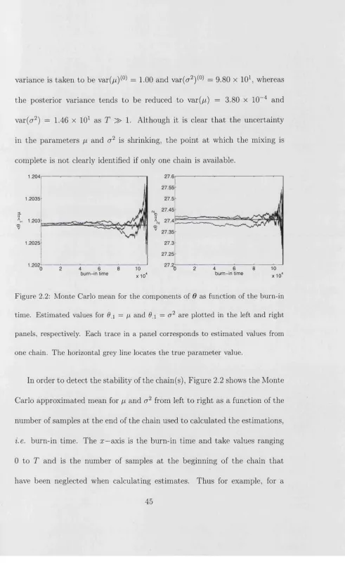
[image:51.598.30.529.28.798.2]variance is taken to be var(/z)^ = 1.00 and var(a2) ^ = 9.80 x 101, whereas the posterior variance tends to be reduced to var(//) = 3.80 x 1CT4 and var(<72) = 1.46 x 101 as T » 1. Although it is clear th at the uncertainty in the parameters [i and <j2 is shrinking, the point at which the mixing is complete is not clearly identified if only one chain is available.
1.204 1.2035
AII
1.203
V
1.2025
1202
0 2 4 6 8 10 0 2 4 6 8 10
b u r n -in tim e x 1 0 * b u m - in tim e x 1 Q ^
Figure 2.2: M onte Carlo mean for the components of 6 as function of the burn-in
tim e. E stim ated values for 9.i = fi and 6.i = a 2 are p lotted in the left and right
panels, respectively. Each trace in a panel corresponds to estimated values from
one chain. The horizontal grey line locates the true parameter value.
In order to detect the stability of the chain(s), Figure 2.2 shows the Monte Carlo approximated mean for // and a 2 from left to right as a function of the number of samples at the end of the chain used to calculated the estimations, i.e. burn-in time. The x—axis is the burn-in time and take values ranging 0 to T and is the number of samples at the beginning of the chain that have been neglected when calculating estimates. Thus for example, for a
[image:52.595.28.519.32.834.2]burn-in time equal to 10 iterations, the mean for the last T — 10 samples states of the chain is plotted. The smaller the sample size, the bigger the
burn-in time and therefore the variation in the estim ated mean. Each trace
for this running mean corresponds in each panel to the estimates of a chain for a given parameter, a horizontal grey solid line locates the true value of
the param eter Q^. Estimation for all three chains seem to stabilise after few iterations for both param eter components. In addition, for 0 2 = &2 one of
the chains tends to be slightly down shifted from the true values but only with an error of 1 x 10⁻² . In all cases, r could be set for a value of less than 2000 iterations. To refine further the value of the burn-in time, zooms of the samples and the Monte Carlo estimates should be made. In the typical case where only one chain is available, burn-in time estim ation is made from
plots like Figure 2.2 but looking only at one chain in isolation. Therefore, convergency assessment by eye can provide unreliable estimates of burn-in
times, which may in tu rn affect the posterior estimates.
The theory described in the last section, assured th a t the chain generated
by the Metropolis-Hastings algorithm in conjuction with the Gibbs sampler
will reach the required target distribution, i. e. the posterior distribution but it does not give any details on when this will happen. Theoretical results are
of the MCMC techniques. Any test th at is used to diagnose convergency
provides a final conclusion when the chain has not reach convergence to the target distribution but conclusions are always ambigouos for complete
convergence. It is common th a t the chain may appear th a t has reached
convergence however there is always the possibility th a t the chain is actually trapped for a finite time in a region or mode of the posterior rather than properly exploring the param eter space [31, 13].
In the MCMC literature, there are available several quantitative tests to diagnose convergency and mixing for a given chain or sets of chains. The
more prominent tests used in several packages and software available for im plementation of MCMC techniques include: Gelman and Rubin (GR) statis
tic [31], Geweke time series test [33], Heildelberger and Welch test [44], and the Raftery and Lewis test [78] among others.
In order to quantify the convergence of the algorithm, the GR statis
tic [31, 95] is used throughout this Thesis to assess convergency in a more quantitative way. If only one chain is available, and is long enough, the GR statistic can be calculated by fragmenting the chain into segments and
consider each of the segments as a chain itself [31, 95, 13].
The GR statistic is based on the idea th a t the best way to identify non- convergency [31, 13] is the simulation of multiple sequences for distinct and
These dispersed points are used as initial conditions for the several chains to be generated. Given th a t the Markov chain is built in such a way th a t
asymptotically the chain states are a sample from the target distribution,
same behaviour. The variance within the chains should be the same as the
variance across the chains [95] for all scalar summaries of interest from the resulting empirical distributions.
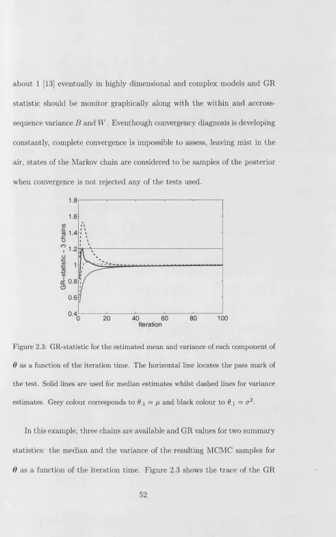
The GR statistic is defined for a single summary statistic of interest. Let £ be the summary statistic, e.g. the sample mean, median, etc. It is assumed there are available c parallel simulations of the same chain, each of length T.