Abstract—This paper proposes a novel algorithm that can be integrated with various design and evaluation tools, to more accurately and rapidly predict stability in multi-bit delta-sigma (Δ-Σ) modulators. Analytical expressions using the nonlinear gains from the concept of modified nonlinearity in control theory are incorporated into the mathematical model of multi-bit Δ-Σ modulators to predict the stable amplitude limits for sinusoidal input signals. The nonlinear gains lead to a set of equations which can numerically estimate the quantizer gain as a function of the input sinusoidal signal amplitude. This method is shown to accurately predict the stable amplitude limits of sinusoids for 2nd-, 3rd-, 4th-, 5th- and 6th-order 3- and 5-level mid-tread quantizer based Δ-Σ modulators. The algorithm is simple to apply and can be extended to midrise quantizers or to any number of quantizer levels. The only required input parameters for this algorithm are the number of quantizer levels and the coefficients of the noise transfer function.
Index Terms—delta-sigma, multi-bit quantizer, nonlinear gains, stability
I. INTRODUCTION
A. Literature review-limitations of existing approaches
The stable input amplitude limits for Delta-Sigma (Δ-Σ) modulators are complicated to predict due to the non-linearity of the quantizer. The stable amplitude limit is defined as the amplitude beyond which the quantizer input exhibits large oscillations before eventually increasing to an exponentially large value. This stable amplitude limit decreases as the order of the Δ-Σ modulator increases. Various techniques have been proposed for predicting the stability of one-bit quantizer based Δ-Σ modulators. One technique is to model the quantizer as a threshold function in the state equations, which gets complicated for higher-order Δ-Σ modulators and is limited to 1st- and 2nd- order Δ-Σ modulators [1]. Another approach to simplify the analysis has been to assume a DC input to the Δ-Σ modulator [2]-[7]. In [8], separate signal and quantization noise nonlinear gains have been used for the stability analysis of 2nd- and 3rd-order Δ-Σ modulators for DC and sinusoidal inputs using the root locus approach. The nonlinear gains have been derived from the concept of modified nonlinearity in nonlinear control theory [9]. This approach of using a quasi-linear technique allows the nonlinear quantizer to be replaced by an equivalent gain, for each of the inputs, i.e. the signal and quantization noise. The linearized modeling approach using nonlinear gains in [8] did not previously provide useful stability predictions, until a new interpretation of the instability mechanism for Δ-Σ modulators based on the quantization noise amplification was given in [10]. However, this is restricted to DC inputs. A combined approach of deploying the separate signal, quantization noise gains in [8], and of the quantization noise amplification in [10] is given in [11], where stability has been predicted for a single-sinusoidal input. In [12], the analysis is extended for predicting stability for dual-sinusoidal inputs. An in-depth analysis of the approach in [11], [12] with detailed simulation results is given in [13]. As the approaches in [11]-[13] are applied to quantify the stability limits of low-pass ∆-Σ modulators, the analysis and results for predicting stability in band-pass ∆-Σ modulators are detailed in [14]. A novel method based on this approach is given in [15]. It quantifies the maximum stability limits in higher-order ∆-Σ modulators for multiple-sinusoidal inputs. It can be observed that all
Jaswinder Lota,
Senior Member,
IEEE, M. Al-Janabi,
Member, IEEE
and Izzet Kale,
Member, IEEE
the reported approaches, to the authors’ best knowledge, relate to the stability of one-bit ∆-Σ modulators. Furthermore, some of these approaches assume DC inputs and/or are restricted to lower-order ∆-Σ modulators [1]-[7], [10].
B. Multi-bit quantizers
Comparatively little work is reported in the open literature on the nonlinear behaviour and stability analysis of multi-bit Δ-Σ modulators. As multi-bit quantization is believed to be accurately modeled by a linear gain and additive white noise, most publications on the stability of multi-bit quantizer Δ-Σ modulators are based on this widely accepted model of [16], [18], [19]. In [16] and [17], stability analysis is undertaken to evaluate robustness against circuit non-idealities rather than on the amplitude of the input signal. Although it is shown in [18] that multi-bit quantization is nonlinear and has a limiting overloading level, the accurate prediction of the stability limits of multi-bit quantizer based Δ-Σ modulators still remains unresolved. A lower-bound has been established in [19] and [20], which however does not consider any of the statistical properties of the quantizer input and its effects on the quantizer gain. The statistical properties of the signal and quantization noise variance at the quantizer input simultaneously determine the quantizer gain. The Δ-Σ modulator therefore becomes interlinked between the signal and the quantization noise transfer functions.
In this paper, the stability prediction of multi-bit Δ-Σ modulators based on the nonlinear gains for multi-bit quantizers is given. The quantizer gain is a function of the quantizer input variance which is challenging to predict as it consists of both the quantization noise and the signal at the input to the quantizer. The quantization noise is henceforth referred to as noise. To accurately predict the quantizer input variance, the Δ-Σ modulator is modeled as two interlinked systems, one for the signal and the other for the noise. The noise model assumes the noise to be Gaussian at the quantizer input, which is a reasonable assumption for higher-order Δ-Σ modulators and/or for multi-level quantizers. The proposed method is able to accurately predict the stable input amplitude limits of higher-order 3-level and 2nd-, 3rd-, 4th-, 5th- and 6th-order 5-level quantizer based Δ-Σ modulators. The method given although linearises the system, predicts the quantizer gain as a function of the input signal. This is accomplished by a novel numerical technique that estimates the quantizer gain as a function of the sinusoidal input signal amplitude for multi-bit quantizers. This technique has been summarized as an algorithm which is straightforward to incorporate into design and simulation tools to speed up the design and evaluation of Δ-Σ modulators. The only parameters required for the algorithm are the number of quantizer levels and the coefficients of the Δ-Σ modulator noise transfer function.
In Section-II, the stability of Δ-Σ modulators is explained in terms of the quantizer gain. The multi-bit quantizer parameters along with the quantizer models for the 3- and 5-level quantizers are given in Section-III. These are used to estimate the quantizer gain as a function of the input signal thus summarizing the proposed novel algorithm. The simulation results are given in Section IV, followed by the conclusions and recommendations in Section V.
II. DELTA-SIGMA MODULATOR STABILITY
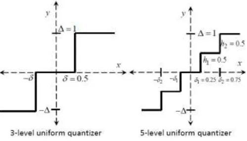
This paper focuses on the stability analysis of 3-level and/or 5-level quantizer based 2nd- to 6th-order Δ-Σ modulators as these would cover a wide range of design specifications and data conversion applications. The quantizer models for the 3-level and 5-level mid-tread uniform quantizers are shown in Fig. 1, where the maximum quantizer output is ±Δ, which is assumed as ± 1. The step rise of the quantizer is given by hm where m = 1, 2,. The points along the x-axis at which the quantizer levels change are
Fig. 1. Mid-tread quantizer models.
Since integration of a random variable tends to make its distribution approach a Gaussian distribution, it is reasonable to assume a Gaussian distribution for the quantizer input for higher-order Δ-Σ modulators. The N-level quantizer gain for a Gaussian input with variance e2is given by [9]:
M
m m m
N h f
K
1
2 (1) where 2 2 2 2 1 ) ( e z e e z f
(2)
and N 2M1.
From (1) and (2), the quantizer gains for the 3-level and 5-level quantizers in Fig.1 are respectively given by:
2 2 2 5 . 0 3 2 2 e e K e
(3)
2
2 2 2 2 75 . 0 2 25 . 0 5 2
1 e e
e e K e
(4)
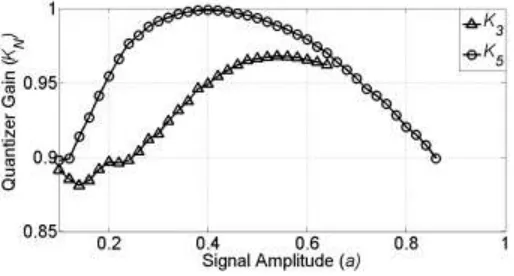
From (3), (4) and measuring the variance e2at the input to the quantizer, one can evaluate KN. For a 4th-order Δ-Σ modulator, the
variation of the quantizer gains K3 and K5with the increase in the sinusoidal input amplitude a are shown in Fig. 2. For the 3-level
quantizer, the 4th-order Δ-Σ modulator is found to be stable up to a = 0.63. The quantizer gain K3 is found to decrease for a <
0.63 indicating the onset of instability and where e 2
is observed to rise exponentially just as a 0.64. For the 5-level quantizer, the 4th-order Δ-Σ modulator is found to be stable up to a = 0.86, beyond which e2 rises exponentially indicating the start of
Fig. 2. Quantizer gain variation.
If one can numerically predict the variation of e 2
as a function of a then the stable amplitude limits can be found by evaluating KN.
III. QUANTIZER INPUT VARIANCE A. Nonlinear quantizer model
The Δ-Σ modulator can be modeled as two interlinked systems, one for the signal and the other for the noise [8]. The signal model with an N-Level (NL) quantizer signal gain KxNL is shown in Fig. 3, where G(z) and H(z) are the Δ-Σ modulator’s signal
and noise transfer functions respectively. The sinusoidal signal input to the Δ-Σ modulator is x(n) and the output signal is yx(n).
The signal at the quantizer input is ex(n) with a variance ex 2
. The noise model with an NL quantizer noise gain KqNL is shown in
Fig. 4, where the noise output of the Δ-Σ modulator is given by yq(n). The quantizer noise input is eq(n) with a variance eq2. The
noise is added to the Δ-Σ modulator loop as additive white noise q(n) with a zero mean and variance q2.
[image:4.612.181.430.467.647.2]Fig. 3. Δ-Σ modulator with signal quantizer gain.
Fig. 4. Δ-Σ modulator with noise gain and additive white noise.
quantizers have been derived in [9] and are used for analysis in this section. The gain derivations for the mid-rise quantizers are also complicated to predict. However, this novel algorithm is equally applicable to mid-rise quantizer based Δ-Σ modulators too. The noise and signal mid-tread quantizer gains KqNL and KxNL are given in [9] as:
1 1 2 2 1 )! 2 ( 2 , 1 , 2 1 1 2 22
F eq m M m m eq qNLh
K
(5)
1 1 2 2 1 )! 2 ( 2 , 2 , 2 1 1 2 22
F eq m M m m eq xNLh
K
(6)where eq a 2
(7)
F1(,, ) is the Confluent Hypergeometric Function of the first kind given by [21] :
.... ! 2 ) 1 ( ) 1 ( 1 ) , , ( 2
1
F (8)
Γ() is a gamma function of [22] and is the index for summation.
The term quantizer henceforth referred to in the analysis would be for the mid-tread quantizer. From (5), (6) and Fig. 1 for a 3-level quantizer δ =δ1 = 0.5, h1 = Δ =1 and M = 1. The noise gain KqNL and signal gain KxNL with these parameters are given by:
Kq3L 2q3L
(9)
Kx3L 2x3L
(10)
where .... , 1 , 2 5 0078 . 0 , 1 , 2 3 1250 . 0 1 , 1 , 2 1 2 1 5 2 1 3 2 1 3
F F F
eq eq
eq L
q (11)
,2, ....
2 5 0078 . 0 , 2 , 2 3 1250 . 0 1 , 2 , 2 1 2 1 5 2 1 3 2 1 3
F F F
eq eq
eq L
x (12)
Similarly from (5), (6) and Fig. 1 for a 5-level quantizer δ1 = 0.25, δ2 = 0.75, h1 = h2 =0.5 and M = 2. The noise gain KqNL and the
signal gain KxNL for the 5-level quantizer are given by:
Kq5L 2q5L
(13)
Kx5L 2x5L
(14)
where .... , 1 , 2 5 020 . 0 , 1 , 2 3 1562 . 0 1 , 1 , 2 1 2 1 5 2 1 3 2 1
5
F F F
eq eq
eq L
.... , 2 , 2 5 020 . 0 , 2 , 2 3 1562 . 0 1 , 2 , 2 1 2 1 5 2 1 3 2 1 5
F F F
eq eq
eq L
x (16)
As seen from (11), (12), (15) and (16), the terms for qNLand xNL and hence the noise and signal quantizer gains differ only in the variables for in F1(,, ), which is consistent with (5) and (6).
B. Noise variance at input to quantizer
From Fig. 4, the noise eq(n) at the quantizer input is given in [8]:
df e H K e H f j qNL f j q eq 2 2 2 2 2 2 ) ( 1 ) (
2 (17)
The numerical analysis in [8] confirms that it is reasonable to assume q(n) to have a uniform PDF. Also under the assumptions that the quantizer is not overloaded and is a multi-bit quantizer (> 2 bits), a uniform PDF provides an acceptable approximation as reported in [23]. In the no-overload region, the noise variance of a multi-bit quantizer with a step size hm and a uniform PDF is
given by: 12 2 2 m q h
(18)
From (18), q 2
is 0.0833 and 0.0208 for the 3- and 5-level quantizers respectively. From (17) and (18), one can determine the variation of eq2 as a function of the noise gain KqNL for a given H(z). The variations in eq2 are investigated for 5-level and 3-level
quantizer based 2nd-, 3rd-, 4th-, 5th- and 6th-order H(z)s and are plotted in Fig. 5a and Fig. 5b respectively. This is done by converting (17) into the time-domain by using Parseval’s theorem and solving it numerically using MATLAB. Alternatively, one can also develop a SIMULINK model for Fig.4. It is observed that eq2 increases as the order of H(z) increases from 2 to 6. As q(n) decreases with the increase in the number of quantizer levels, the noise variance eq
2
at the input to the quantizer also decreases for the same noise gain and H(z) order. Since the NTF(z) is a high-pass transfer function, H(z) is correspondingly a low-pass transfer function which amplifies the noise in the baseband. As KqNL decreases, the suppression of noise degrades and
eq2 increases leading to a fall in the Signal-to-Noise Ratio (SNR) in the baseband. This indicates the onset of instability, i.e. the
noise accordingly shifts towards the baseband region as KqNL decreases [8].
C. Quantizer input variance and signal amplitude
As the signal and noise are uncorrelated, the combined variance at the quantizer input is given by the sum of the variance of the quantizer noise and the quantizer signal input. These are determined in this section. From (9) and (13), for the 3-level and 5-level mid-tread quantziers, the following expressions are obtained:
2q3LKq3L 0
(19)
2q5LKq5L 0
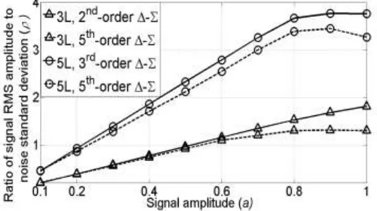
(20) From (19), (20), the values obtained in Fig. 5 for KqNL and eq2 can be used to solve for . The values of for the 3- and 5-level
[image:7.612.174.442.289.439.2]quantizers are shown in Fig. 6. As the noise variance at the quantizer input is higher for a higher-order Δ-Σ modulator for the same signal amplitude a, lower values are obtained for the 5th-order as compared to the 2nd- or 3rd-order for the 3- and 5-level quantizers. Higher values of are obtained for the 5-level quantizer as compared to the 3-level as the quantization noise is lower for the 5-level quantizer as compared to the 3-level for the same signal amplitude.
Fig. 6. Ratio of signal RMS amplitude to noise standard deviation versus the signal amplitude for 3- and 5-level Δ-Σ modulators.
From the values of , eq and (10), (14) one can obtain the values of KxNL. From Fig. 3, assuming that integrators are used in the
Δ-Σ modulators G(z)1, therefore:
xNL x
K
z
X
z
E
1
)
(
)
(
(21)
From (21):
2
2
2a
2x
K
exNL
(22)From (22), one can obtain the signal variance at the input to the quantizer with a change in the signal amplitude a:
2
2
2 2
NL ex
x
K
a
The signal variance at the quantizer input can be obtained using (23). The corresponding curves for the 3rd- and 5th-order 5-level Δ-Σ modulators are shown in Fig. 7.
Fig.7. 3rd- and 5th-order 5-level mid-tread Δ-Σ modulator’s quantizer signal input variance.
As the signal and noise are uncorrelated, the combined variance at the quantizer input is given by:
e2 ex2 eq2 (24)
From (24), the increase in the combined quantizer input variance for the signal and noise, e2, with the increase in signal
amplitude can be determined. The numerically predicted variance for the signal and noise for the 5-level quantizer input for a 6th -order Δ-Σ modulator is shown in Fig. 8.
Fig.8. 6th-order 5-level Δ-Σ modulator quantizer input variance.
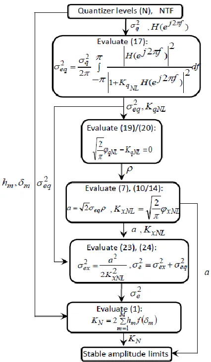
D. Algorithm summary
Fig. 9. Flowchart of the Proposed Algorithm
IV. SIMULATION AND EXPERIMENTAL RESULTS
This section gives the simulation results in Matlab. Subsequently the step-by step values obtained from the algorithm in Fig.9 are given which are validated for an actual prototype design of a 2nd-order 5-level Δ-Σ modulator for WCDMA.
A. Simulation Results.
Fig.10. Fourth-order Δ-Σ modulator in CAFB topology.
The coefficient values for the Δ-Σ modulators are shown in Table I. The coefficients were obtained using Schrier’s MATLAB based Δ-Σ toolbox in [24]. The NTF(z) values are given in the Appendix.
TABLEI
COEFFICIENTS FOR Δ-ΣMODULATORS
Δ Σ i 1 2 3 4 5 6 7
6th-order
δi 0.0003 0.0055 0.0423 0.2001 0.6104 1.1151 1.0000
αi 0.0003 0.0055 0.0423 0.2001 0.6104 1.1151 -
γi 0.0001 0.0011 0.0021 - - - -
5th-order
δi 0.0035 0.0400 0.2127 0.6491 1.1670 1.0000 -
αi 0.0035 0.0400 0.2127 0.6491 1.1670 - -
γi 0.0007 0.0020 - - - - -
4th-order
δi 0.0189 0.1569 0.5683 1.1060 1.0000 - -
αi 0.0189 0.1569 0.5683 1.1060 - - -
γi 0.0003 0.0018 - - - - -
3rd- order
δi 0.0865 0.4675 1.0368 1.0000 - - -
αi 0.0865 0.4675 1.0368 - - - -
γi 0.0014 - - - -
2nd -order
δi 0.4715 1.2364 1.0000 - - - -
αi 0.4715 1.2364 - - - - -
γi 0.0008 - - - -
The simulations undertaken are for a sinusoidal input with a frequency of 8 kHz with a sampling frequency of 512 kHz for an Over-Sampling Ratio (OSR) of 32. All the initial conditions of the Δ-Σ modulators are set to zero. The signal amplitude a is increased from 0 to 1 in steps of 0.01 and the corresponding variance of the quantizer input is measured. From (3), K3 is plotted
in Figs 11 (a)-(d) for the 3-level quantizer for e2 obtained via simulations and compared with the numerical values obtained from
(24) using the proposed algorithm. The numerical values provide a close match to the values obtained via simulations. The simulated values are obtained until the stable amplitude limits of a are reached. However, the numerical values plotted are the theoretical values up to the full scale quantizer input of a =1. It is observed that the higher is the Δ-Σ modulator order, the steeper is the rate at which K3 decreases. The simulated stable amplitude limits are taken until the input to the quantizer begins to rise
exponentially and at this point the simulated K3commences to decrease in value. The numerically computed stable limits of a
correspond to when the numerical value of K3just begins to decrease.
Fig. 11(c). 4th-order Δ-Σ modulator Fig. 11(d). 3rd-order Δ-Σ modulator
From (4), K5 is plotted in Figs 12 (a)-(d) for the 5-level quantizer for e2 obtained via simulations together with those numerical
values obtained from (24) by using the proposed algorithm. The numerical values obtained seem to be sufficiently close to the values obtained via simulations. As with the 3-level case, the simulations are performed up to the stable amplitude limits of a, while the numerical values are plotted for the full scale input amplitude range. The stable amplitude limits are taken until the input to the quantizer begins to rise exponentially and at this point the simulated K5decreases by about 10% of its maximum
value. There is a divergence in the simulated and theoretical values for a < 0.3. This may be attributed to the artefacts of the numerical method used for low input amplitudes such as convergence issues. However the two curves converge rapidly for values a 0.3 in the region of higher amplitude which is critical for predicting the stable amplitude limits.
Fig. 12(a). 6th-order Δ-Σ modulator Fig. 12(b). 5th-order Δ-Σ modulator
The numerically stable amplitude limits values are given in Table II where Δe indicates the absolute error between the simulated
and the numerically predicted limits of a.
TABLEII
SIMULATION VALUES
Multi-bit quantizer Order Stable Limit
Δe
3-level
Simulated Numerically Predicted
II 0.92 0.68 0.24
III 0.87 0.71 0.16
IV 0.64 0.60 0.04
V 0.46 0.50 0.04
VI 0.37 0.41 0.04
5-level
Order Stable Limit
Simulated Numerically Predicted
II 0.95 0.88 0.07
III 0.92 0.89 0.03
IV 0.86 0.90 0.04
V 0.79 0.83 0.04
VI 0.75 0.71 0.04
As observed from Table II the algorithm is able to accurately predict the stable amplitude limits for multi-bit Δ-Σ modulators. The errors between the simulated and numerical values Δe are reduced as the order of the Δ-Σ modulator increases because the
quantization noise becomes more Gaussian. Also as the quantization noise becomes more Gaussian and the number of quantizer levels is increased from 3 to 5, there is a decrease in Δe. The errors are below 0.1 for the 4th- and higher-orders for the 3-level
quantizer case. They are also below 0.1 for 2nd- to 6th-orders for the 5-level quantizer case. B. Step-by step experimental validation
This section gives the step-by step values obtained in the algorithm given in Fig. 9 for a 2nd-order five-level quantizer Δ-Σ modulator developed for WCDMA applications in 90 nm CMOS. The stable input amplitude for the Δ-Σ modulator is given in [25] as 0.794 beyond which the SNR starts to fall. The stable amplitude limit obtained from the numerical method is 0.880, for which the error is 0.080. The step-by step values are given in Table III. The starting point for the algorithm is the noise transfer function H(z)=(1-z-1)2and the quantizer levels N =5. As the maximum level of the quantizer is Δ = 1, for a five-level quantizer corresponding to this q2 can be generated as being uniformly distributed between 0.25. Accordingly (17) is evaluated that
gives the variation of e with Kq5L which for 0.153 is 1.027. One can then evaluate (20) which gives the value of =4.050.
Tracing the further intermediate values obtained from (7), (14) gives the signal quantizer gain as Kx5L= 1.053 which corresponds
to the signal amplitude a = 0.880, which is the value at which the quantizer gain falls to 10% of its maximum value which is 0.930 and therefore taken as the numerically evaluated stable amplitude limit. The SNR variation with the signal amplitude for the prototype Δ-Σ modulator are given in [25] for a signal frequency of 448 kHz and the sampling frequency of 76.8 MHz and the WCDMA bandwidth of 1.94 MHz. The SNR increases to 62 dB for the signal amplitude of -2.5 dBFS. The SNR commences to fall at the signal amplitude of -2 dbFS, indicating the signal amplitude as 0.794, beyond which the Δ-Σ modulator becomes unstable.
TABLEIII
Quantizer levels 5 H(z) = (1-z-1)2 -
Evaluate (20) = 4.050
Evaluate (7), (14) Kx5L= 1.053 a = 0.88stable amplitude
Evaluate (23), (24) ex2
= 0.349 e2 = 0.373 Evaluate (1) Kq5L = 0.930
V. CONCLUSIONS
A novel method that uses the nonlinear quantizer gains to accurately predict the stability of multi-bit Δ-Σ modulators for sinusoidal inputs has been reported. As the model used assumes a Gaussian noise at the quantizer input, the accuracy of the method increases for higher-order Δ-Σ modulators for the 3-level quantizer case and for 2nd- to 6th-order Δ-Σ modulators for the 5-level quantizer case. The quantizer gain is found to decrease as the signal amplitude increases. As the Δ-Σ modulator is modeled as an interlinked system of signal and noise transfer functions, the decrease in quantizer gain can be numerically evaluated as a function of the signal amplitude. As the quantizer gain decreases, the input variance to the quantizer increases whereby eventually it rises exponentially as the Δ-Σ modulator becomes unstable. The reported prediction method involves the solutions of nonlinear equations, which have been summarized as an algorithm and can be extended to any number of quantizer levels. The algorithm is verified for a prototype five-level Δ-Σ modulator developed for WCDMA applications in 90nm CMOS. The algorithm can be integrated in various design tools to predict more accurately and rapidly stability in multi-bit Δ-Σ modulators for sinusoidal inputs. The only required inputs for the algorithm are the number of quantizer levels and the Δ-Σ modulator noise transfer function. The stability analysis for dual-tone and multiple sinusoids for multi-bit Δ-Σ modulators are underway and would be reported in a future publication.
APPENDIX TABLEA
Δ Σ Noise Transfer Function H(z)
6th-order
(z2 - 2z + 1) (z2 - 1.999z + 1) (z2 - 1.998z + 1) --- (z2 - 1.509z + 0.5722) (z2 - 1.595z + 0.6629) (z2 - 1.782z + 0.8595)
5th-order
4th-order (z
2 - 2z + 1) (z2 - 1.998z + 1)
--- (z2 - 1.332z + 0.4552) (z2 - 1.562z + 0.7166)
3rd- order (z-1) (z
2
- 1.999z + 1) --- (z-0.5934) (z2 - 1.37z + 0.5825)
2nd -order (z
2 - 1.999z + 1)
--- (z2 - 0.7636z + 0.236)
REFERENCES
[1] S. Hein, and A. Zakhor, “On the stability of sigma-delta modulators”, IEEE Trans. on Signal Processing, vol. 41, no.7, pp. 2322-2348, Jul 1993.
[2] P, Steiner, and W. Yang, “Stability analysis of the second-order sigma-delta modulator”, Proc. IEEE Int. Symp. Circuits Syst., vol. 5, pp. 365-368, 1994.
[3] N. A. Fraser, and B. Nowrouzian, “A novel technique to estimate the statistical properties of sigma-delta A/D converters for the investigation of DC stability”, Proc. IEEE Int. Symp. Circuits Syst., vol.3, pp.111-289-111-292, May 2002.
[4] N. Wong, and N.G. Tung-Sang, “DC stability analysis of higher-order, lowpass sigma-delta modulators with distinct unit circle NTF zeroes”, IEEE Trans. on Circuits & Syst.-II, vol. 50, issue 1, pp. 12-30, Jan 2003.
[5] J. Zhang, P.V. Brennan, D. Juang, E. Vinogradova, and P.D. Smith, “Stable boundaries of a 2nd-order sigma-delta modulator”, Proc. South. Symp. Mixed Signal Design, Feb 2003.
[6] J. Zhang, P.V. Brennan, D. Juang, D, E. Vinogradova, and P.D. Smith, “Stable analysis of a sigma-delta modulator”, Proc. IEEE Int. Symp. Circuits Syst., vol.1, pp.1-961-1-964, May 2003.
[7] D. Reefman, J.D. Reiss, E. Janssen, and M.B. Sandler, “Description of limit cycles in sigma-delta modulators”, IEEE Trans. on Circuits and Syst-I., volume 52, issue 6, p.1211 – 1223, June 2005.
[8] S. H. Ardalan, and J.J. Paulos, “An analysis of non-linear behaviour in Σ-Δ modulators”, IEEE Trans. on Circuits and Syst., vol. CAS-34, no. 6, pp. 1157-1162, Jun 1987.
[9] D. P. Atherton, Nonlinear Control Engineering: Describing Function Analysis and Design. London, U.K. Van Nostrand Reinhold, 1982, pp. 383–388.
[10] L. Risbo, “Stability predictions of higher-order delta-sigma modulators based on quasi-linear modeling”, Proc. IEEE Int. Symp. on Circuits and Syst., vol.5, pp. 361-364, 30 May-02 Jun 1994.
[11] J. Lota, M. Al-Janabi, and I. Kale, “Stability analyses of higher-order delta-sigma modulators using the Describing Function method”, Proc. IEEE Int. Symp. on Circuits and Syst., pp. 593-596, May 2006.
[12] J. Lota, M. Al-Janabi, and I. Kale, “Stability analyses of higher-order delta-sigma modulators for dual-sinusoidal inputs”, Proc. IEEE Inst. and Measurements Tech. Conf., Warsaw, Poland, pp. 1-5, May 2007.
[13] J. Lota, M. Al-Janabi, and I. Kale, “Nonlinear stability analyses of higher-order sigma-delta modulators for DC and sinusoidal inputs”, IEEE Trans. on Inst. and Measurements, vol. 57, no. 3, pp. 530-542, Mar 2008.
[14] D.G. Altinok, M. Al-Janabi, M., and I. Kale, “Stability analysis of bandpass sigma-delta modulators for single- and dual-tone sinusoidal input”, IEEE Trans. on Inst. and Measurements, vol. 60, issue 5, pp. 1546-1554, Feb 2011.
[15] J. Lota, M. Al-Janabi, and I. Kale, “Nonlinear stability analyses of higher-order sigma-delta modulators for multiple-sinusoidal inputs’, IET Journal of Ckts., Devices and Syst., Mar 2012.
[17] M. Ranjbar and O. Oliaei, “A Multibit Dual-Feedback CT Delta Sigma Modulator with Lowpass Signal Transfer Function,” IEEE Trans. Circuits Syst.-I, vol. 58, no. 9, pp. 2083–2095, Sep 2011.
[18] R. Baird and T. Fiez, “Stability analysis of high-order delta-sigma modulation for ADCs,” IEEE Trans. Circuits Syst.-II, vol. 41, no. 1, pp. 59–62, Jan 1994.
[19]Lokken, A. Vinje, T. Saether, and B. Hernes, “Quantizer nonoverload criteria in sigma-delta modulators,” IEEE Trans. Circuits Syst.-II, vol. 53, no. 12, pp. 1383–1387, Dec 2006.
[20] P. Kiss, J. Arias, D. Li, and V. Boccuzzi, “Stable high-order delta-sigma digital-to-analog converters,” IEEE Trans. Circuits Syst.-I, vol. 51, no. 1, pp. 200–205, Jan 2004.
[21] Athanasios Papoulis, Probability, Random Variables, and Stochastic Processes. New York, London, McGraw-Hill 1965.
[22] M. Abramowitz and I. A. Stegun, Handbook of Mathematical Functions. New York: Dover Publications, 1970.
[23] R. Gray, “Quantization noise spectra ”, IEEE Trans. on Information Theory, , volume 36, no.6, p.1220 – 1224, Nov1990.
[24]R. Schreier, High-level design and simulation of delta-sigma modulators. Delta-Sigma Matlab Toolbox, Jul 2009. Available at: www.mathworks.com/matlabcentral/fileexchange/19