Munich Personal RePEc Archive
A Semi-Analytical Parametric Model for
Dependent Defaults
Balakrishna, B S
16 August 2006
Online at
https://mpra.ub.uni-muenchen.de/14918/
A Semi-Analytical Parametric Model for Dependent Defaults
B. S. BALAKRISHNA∗
August 16, 2006, Revised: May 15, 2007
Abstract
A semi-analytical parametric approach to modeling default dependency is presented. It is a multi-factor model based on instantaneous default correlation that also takes into account higher order default correlations. It is capable of accommodating a term structure of default correlations and has a dynamic formulation in the form of a continuous time Markov chain. With two factors and a constant hazard rate, it provides perfect fits to four tranches of CDX.NA.IG and iTraxx Europe CDOs of 5, 7 and 10 year maturities. With time dependent hazard rates, it provides perfect fits to all the five tranches for all three maturities.
Credit derivatives market has grown rapidly in recent years in response to the growing need for transferring and hedging credit risk. Growing innovations in this market has made understanding these products more urgent than ever. Various models have been developed to understand the role of default correlation on the prices of such products referencing a portfolio of underlying assets. A method for pricing these correlation products that has become standard is based on the Gaussian copula. There are some well known shortcomings in this approach. It deals effectively with default time correlation rather than default correlation itself. There is no straightforward way to accommodate correlation term structures. The correlation smile implied from the market is quite significant, an indication that the method is inadequate to price nonstandard products. These and other issues have been discussed by various authors, for instance by Finger [2004], Friend and Rogge [2004], Gregory and Laurent [2004], Hager and Sch¨obel [2005]. Better models addressing these issues have also been developed. Some recent work in this direction involves implying the copulas by Hull and White [2006], modeling the distance to default variables as in Albanese, Chen and DAlessandro [2005], Baxter [2006], modeling the default intensities as in Joshi and Stacey [2005], Chapovsky, Rennie and Tavares [2006], Errais, Giesecke and Goldberg [2006], and modeling the loss distributions as in Bennani [2005], Sidenius, Piterbarg and Andersen [2005], Sch¨onbucher [2005], Brigo, Pallavicini and Torresetti [2006].
Here in this article, a semi-analytical parametric multi-factor model for pricing such correlation products is discussed incorporating default correlation rather than default time correlation. Being based on instantaneous default correlation, it is capable of handling correlation term structures in addition to a term structure of default probabilities. It also takes into account higher order default correlations in terms of a parameter that could explain clustering tendency of credit defaults. It has a dynamic formulation in the form of a continuous time Markov chain that has the potential to be useful for further development.
It is based on conditional independence of defaults at differing times. That is, if a credit name has survived an instant, an event at that instant does not have any further influence on the credit name. All defaults associated with an event would occur instantaneously at the same instant as
∗
that of the event. Simultaneous defaults have been discussed before, see for instance Duffie and Singleton [1999]. It is a characteristic feature of the so called shock models based on Marshall-Olkin copula that have been in use in reliability theories. Here we present a self-contained, a more convenient and an instantaneous approach to modeling such default dependencies, attempting to extract its power by formulating it in a parametric setting. A semi-analytical representation of the default probability distribution for a homogeneous collection of credit names lets us price CDOs accurately and efficiently using arbitrary precision arithmetic. A two factor model with four free parameters and a constant hazard rate is used to provide perfect fits to the four non-equity tranches of CDX.NA.IG and iTraxx Europe CDOs of 5, 7 and 10 year maturities. Allowing for time varying hazard rates obtains perfect fits to all the five tranches of both CDX.NA.IG and iTraxx Europe CDOs for all three maturities. These fits could be useful for hedging purposes and pricing non-standard instruments.
First, some results are derived in section 1 for the intermediate objects involved in this approach, followed by a factor based approach to motivating and building the model in a multi-factor setting for a general collection of credit names. Section 2 discusses the multi-factor model for homogeneous credit names, specializes to two factors, and provides fits to CDX.NA.IG and iTraxx Europe CDO tranches. Section 3 discusses a dynamic formulation of the model in terms of a continuous time Markov chain. Section 5 discusses a scaled correlation model potentially applicable for heavily correlated collections with non-uniform hazard rates. Section 6 concludes with some remarks.
1
Modeling Simultaneous Defaults
Let us first derive some results that follow from the assumption of conditional independence of defaults at differing times. Considerncredit names,i= 1, ..., n, with default timesτi’s and hazard
ratesλi(t)’s. Let
Q(t1, ..., tn) = Prob(τ1> t1, ..., τn> tn) (1)
be the joint survival probability up to times t1, ..., tn. As assumed, given that credit namesi and
j have survived up to timesti and tj respectively,ti 6=tj, their respective defaults at ti and tj are
independent of each other. Under this assumption,Qcan be expressed as
LnQ(t1, ..., tn) =− n
X
i=1
Z t(i)
t(i−1)
dt π(i)...(n)(t), (2)
where t(i)’s are ordered times, 0 = t(0) ≤ t(1) ≤ ... ≤ t(n), and (i) refers to the credit name associated with the ith ordered time. π
ij...(t)dt is the conditional probability that at least one of
the names in the list{i, j, ...}defaults during the interval (t, t+dt) (unlisted names are not looked at). Note that 1−πij...(t)dt is the conditional probability that the listed names do not default during (t, t+dt) (unlisted names are not looked at). Hence, under our assumption of conditional independence of defaults at differing times, the above expression forQcan be obtained by building it up infinitesimally from t = 0 to tn as a product of terms of the form 1−π(i)...(n)(t)dt. It can also be derived directly from our assumption as detailed in appendix A. It turns out this joint survival probability in fact corresponds to the multi-variate version of the Marshall-Olkin copula in a convenient representation and generalized to time dependent conditional probability densities. For a discussion of such shock models as applied to credit risk, see Duffie and Singleton [1999], Elouerkhaoui [2003], Lindskog and McNeil [2003].
Theπdensity is related topij...(t)dt, the conditional probability that all the listed names default during (t, t+dt) (unlisted names are not looked at). First three of these relations are
πij(t) = pi(t) +pj(t)−pij(t),
πijk(t) = pi(t) +pj(t) +pk(t)−pij(t)−pik(t)−pjk(t) +pijk(t). (3)
Remaining relations can analogously be written down. The two-point default probability density lets us express the instantaneous correlation ρij(t) between credit names iand j as
ρij(t) = q pijdt−(pidt)(pjdt)
pidt(1−pidt)pjdt(1−pjdt) ≈
pij(t)
q
λi(t)λj(t)
. (4)
If say λi(t) ≤ λj(t), ρij(t) has an upper bound of qλi(t)/λj(t). This is because pij(t)/λi(t), conditional probability of finding credit name j defaulted during (t, t+dt) knowing that i has defaulted, should not exceed unity. Note that ρij(t) can be interpreted as
q
λi(t)/λj(t) times that
probability. Negative correlations are not supported.
Given the joint survival probability, we can get the joint survival and default probability Pij.... This is the probability that the names listed in {i, j, ...} default before their times, that is τi < ti, τj < tj, ..., while the others survive up to their times. Probability that no names default before
their times is of course given by Qitself. The others are related to Qas
Pi(t1, ..., tn) = Qi−Q,
Pij(t1, ..., tn) = Qij−Qi−Qj+Q,
Pijk(t1, ..., tn) = Qijk−Qij−Qik−Qjk+Qi+Qj+Qk−Q. (5)
Remaining relations can analogously be written down. Qij...is obtained fromQ(t1, ..., tn) by setting
ti, tj, ...to zero for the names in the list{i, j, ...}. The dependence ofQij...’s on the remaining times is not shown for simplicity. If those times are all the same, say t, then we have from (2)
LnQij...(t) =−
Z t
0
ds π6=ij...(s), (6)
where{6=i, j, ...}lists out the names not in{i, j, ...}. For a homogeneous collection of credit names, equation (5) for the probabilityPij... having ν names in the list {i, j, ...}gets simplified to
P[ν]=
ν
X
k=0
(−1)k(νk)Q[ν−k]=
ν
X
k=0
(−1)k(νk) exp
−
Z t
0
ds π[n−ν+k](s)
, (7)
where only the number of names are shown as subscripts. When concerned with just the number of defaults, this should be multiplied by the number of combinations of ν out of ncredit names.
Thus, in general, if we have a model or some prescription for determining pij...(t)’s, we can use them in (3) to determineπij...(t)’s that can be used in (6) to determineQij...(t)’s which in turn can be used in (5) to determine Pij...(t)’s. Pij...(t)’s are useful in pricing multi-name credit products.
For instance, for a νthto default credit product, we need to know the probability that less than ν
names have defaulted beforet. This is given by
Q+X
i
Pi+X
ij
Pij +X
ijk
Pijk+...+
X
ijk...
Pijk..., (8)
Let us now introduce a parametric model for dependent defaults. As a motivation, let us assume that the collective dynamics is governed bymevent types called factor names, that are independent of each other capable of generating events potentially causing joint defaults. Because joint arrivals of such independent events during an infinitesimal interval (t, t+dt) have probabilities of order(dt)2 or higher, they would be treated individually.
Let as assume for the moment that a credit default during (t, t+dt) implies that a factor name has generated an event during that interval. Letζr(t)dt be the conditional probability that factor
namer generates an event during (t, t+dt). Letγir(t) be the conditional probability of findingith credit name defaulted knowing that factor name r has generated an event during (t, t+dt). This suggests thatλi(t)dt gets a contributionγir(t)ζr(t)dt from therth factor name. Adding up similar
contributions from other factor names, we get1
λi(t) =λi(t) + m
X
r=1
γir(t)ζr(t), (9)
where an additional contribution λi(t) is included, coming from relaxing our assumption that a
credit default implies that a factor name has generated an event. All name-specific contributions toλi(t) are expected to be included in λi(t). Under the assumption that credit names are condi-tionally independent given that an event of certain type has arrived, we can express the conditional probability density of joint defaults during (t, t+dt) as
pij...(t) = m
X
r=1
(γir(t)γjr(t)...)ζr(t). (10)
There are no additional terms here, since name-specific contributions to joint defaults during (t, t+
dt) are of order(dt)2 or higher, and all order(dt) contributions are expected to be taken care of by a sufficient number of factor names. With these pij...(t)’s, one could sum up the terms in the expansion of πij...(t) in (3) to obtain
πij...(t) =X
k
λk(t) + m
X
r=1
ζr(t)
"
1−Y
k
(1−γkr(t))
#
, (11)
where kruns over only those credit names that are in the subscripted list {i, j, ...}. This can also be obtained directly by noting that the first term is the contribution from name-specific issues and the term under square brackets is the probability that at least one of the names defaults during (t, t+dt) given that an event of typer has arrived.
If λi(t)’s are inputs to the model, equation (9) can be used to implyλi(t). Because λi(t)’s can not be negative, it places a constraint on the parameters γ’s and ζ’s. As for the instantaneous correlation ρij(t) between credit namesiand j discussed earlier, we have
ρij(t)qλi(t)λj(t) =
m
X
r=1
γir(t)γjr(t)ζr(t). (12)
These correlations could be treated as inputs to the model constraining the parametersγ’s and ζ’s further, or this equation could be considered simply as defining implied correlations.
1Such a break up of the hazard rate has been considered before by various authors, as in, for example, Duffie and
2
Homogeneous Credit Names
The above formalism simplifies in the case of a homogeneous collection of credit names. Dropping the credit name subscripts but retaining those for the factor names, equations (9) and (12) read
λ(t) = λ(t) +
m
X
r=1
γr(t)ζr(t),
ρ(t)λ(t) =
m
X
r=1
γr(t)2ζr(t). (13)
For the higher order conditional probability densities, we have2
pij...(t) =
m
X
r=1
γr(t)νζr(t), (14)
whereν is the number of names listed in {i, j, ...}. Equation (11) for theπ-densities simplfies to
πij...(t) =νλ(t) +
m
X
r=1
ζr(t) [1−(1−γr(t))ν]. (15)
As noted earlier, these can be used (7) to determine the joint default probability distribution useful in pricing multi-name credit products. It is also useful to introduce γ(t) through the definition
γ(t) =
Pm
r=1γr(t)2ζr(t)
Pm
r=1γr(t)ζr(t)
. (16)
Note that the numerator above is ρ(t)λ(t) and the denominator is λ(t)−λ(t). Because λ(t) can not be negative this impliesρ(t)≤γ(t)≤1.
The conditional probabilityχν(t) forν ≥3 of finding an additional credit name defaulted during (t, t+dt) knowing that ν−1 of them have defaulted during that interval is
χν(t) =
Pm
r=1γr(t)νζr(t)
Pm
r=1γr(t)ν−1ζr(t)
. (17)
This could be referred to as default cluster coupling and could explain the clustering tendency of credit defaults known as default contagion. It is related to higher order correlations present in the model, namely the instantaneous correlation between a credit name and a cluster ofν−1 names. It is expected to increase with the number of credit names in the cluster. This is not the case with the one-factor model, but naturally holds in multi-factor models. One can prove thatχν(t)≥χν−1(t), with the equality holding only when nonzero γr(t)’s, r = 1, ..., m, are all the same, in which case the model effectively reduces to one-factor. The largest valueχν(t) takes isχn(t) for then−name cluster, which itself has an upper bound given by the largest of γr(t), r = 1, ..., m, as can be seen
by takingn→ ∞. The smallestχν(t) is χ3(t) for a 3−name cluster, that has a lower bound given by γ(t). Because γ(t) ≥ ρ(t), cluster coupling is never less than ρ(t), the probability of a second default knowing the first. An explanation is, two or more defaults during the same infinitesimal interval (t, t+dt) (in reality, during a short period) is an indication that common factors, rather
2It is interesting to observe here that this multi-factor expansion of the conditional probability densities is
math-ematically natural being just an expansion in simple poles along the positive real line in the complexz−plane of the generating functionP∞
ν=1p[ν]zν
−1
than name-specific issues, are more likely to be the causes. In our terminology, factor names, rather than λ(t)’s, are likely to be causing the defaults. However, such contagious features as jumps in hazard rates are not apparent in these types of models because all clustering of defaults takes place instantaneously. Information driven default contagion exhibiting such features has been discussed before in Giesecke [2001] and Sch¨onbucher [2003] in different contexts. For alternate mechanisms, see Davis and Violet [2000] and Jarrow and Yu [2000].
Apart from λ(t), there are 2m parameters in the model, γr(t) and ζr(t), r = 1, ..., m, to be
determined empirically. It is illustrative to use the parameterizationρ,γr, r= 1, ..., mand θs, s= 1, ..., m−1 such that
ζr<m = ρλ
γ2
r
cos2θr r−1
Y
s=1
sin2θs, ζm= ρλ
γ2
m m−1
Y
s=1
sin2θs. (18)
Note that√ρλis the magnitude andθs’s are the angles of am−dimensional vector with components
γr√ζr, r= 1, ..., m. During calibration of the model at the computation level, it is convenient use x0 and xr’s, along with θs’s, related to the model parameters via the relations ρ = γx0 and
γr =x1x2...xr with the box constraints
0≤xr ≤1, r= 0, ..., m, 0≤θs≤ π
2, s= 1, ..., m−1. (19)
In particular, for the two factor model, it is convenient use x0, x1, x2 and θ such that ρ = γx0,
γ1 =x1,γ2 =x1x2, and
ζ1=
ρλ γ2 1
cos2θ, ζ2=
ρλ γ2 2
sin2θ, 1
γ =
1
γ1
cos2θ+ 1
γ2
sin2θ. (20)
Note that γ1 ≥ γ ≥ γ2. Hence γ1 is the upper bound on the cluster coupling discussed earlier. Angleθdetermines the contribution of the second factor. It also controls the distribution of cluster coupling over cluster sizes from three ton, that decreases asθincreases from a uniformγ1 forθ= 0 to a uniform γ2 for θ =π/2. For θ 6= 0, π/2, the intermediate distribution increases with cluster size fromγ1cos2θ+γ2sin2θfor a 3−name cluster to its limiting valueγ1for a largen−name cluster. Computations are done using equation (7). This involves summing up a lot of exponentials with alternating signs that requires great care to ensure that significance is not lost due to machine limitations. In fact, using the popular computers, it is difficult to go beyond the equity tranche. It is safer to use arbitrary precision arithmetic to get to the remaining ones. Arbitrary precision software is readily available and their use lets us price CDOs efficiently. Simplified results for homogeneous names useful in the computations are presented in Appendix B.
A one-factor model does not suffice to provide a good fit to more than two of the CDO tranches. Apart fromλ(t), it has two parameters, ρ(t) andγ(t), and can provide a fit to two of the tranches. It is not able to capture the market perceptions when pricing more than two tranches, perhaps because the tranches are sensitive to a richer correlation structure. Obviously more than two parameters are needed and these are supplied by multi-factor models, in particular a two-factor model chosen for the following analysis.
There are however significant differences with the predicted upfront fees for the equity tranches. The discrepancies become severe as we go to higher maturities. Going to three factors does not appear to provide much improvement. Other choices for the recovery rate give different parameter values, but don’t seem to affect the quality of the fits. The origin of the discrepancies lies in our assumption of a constant hazard rate. An increasing index spread term structure suggests an increasing time dependence for the hazard rate. A constant hazard rate makes defaults more likely at earlier times than as indicated by the index spreads. An increasing time dependence for the hazard rate should give better prices for the equity tranches.
Table 2 presents the results assuming a log-linear time-dependence for the hazard rate, λ(t) =
λ(0)exp(κλt) and the same time dependence for ζr(t)’s maintaining their proportionality to λ(t)
according to (20). For ease of computations, the hazard rate is discretized to be piecewise constant annually withλ(0) the first year multiplied by exp(κλ) year to year. The presence of an additional parameterκλenables us to calibrate the model to all the five tranches. Supporting our observations
above, the model gets calibrated perfectly to all the five tranches, for both CDX.NA.IG and iTraxx Europe CDOs and for all three maturities. Of course, a log-linear hazard rate is not expected to realistically describe the term structure of index spreads. Its purpose here is just to identify an effective hazard rate time dependence that consistently prices the CDO tranches along with the index CDS of the same maturity. When the hazard rate term structure is exogenously supplied, an additional free parameter is not available for calibration. Under such circumstances, it may not be possible to get a perfect fit, but an acceptable best fit could still be possible.
The model is in principle capable of handling a term structure of default probabilities and default correlations. However, implying such term structures from the market data can be a challenging task, and it would be too ambitious to look for a well-behaved perfect fit calibrated simultaneously to all the maturities. One may look for a best fit assuming a continuous hazard rate term structure that is log-linear in-between maturities, and term structures for the other parameters that are piecewise constants, so that only the first maturity log-linear coefficientκλ is additionally available for calibration. An attempt in this direction, though successful, resulted in significant discrepancies, perhaps suggesting that it is important to include bid-ask spreads during calibration or have a more flexible model of the term structure of hazard rates.
Figure 1 shows the joint default probability distribution as a function of the number of defaults over a time period of 5, 7 and 10 years using the model parameters from Table 2 calibrated to iTraxx Europe CDOs of the corresponding maturities. The distribution has a large body of mass contributing mainly to the first few tranches. As we go to higher maturities, this body of mass moves to the right contributing more and more to the remaining tranches. The shape of this mass is largely determined by the term structure of hazard rates. For low maturities such as 5 year, it affects mainly the equity tranche. This explains why we are able to get realistic values for the model parameters assuming a constant hazard rate and calibrating to only the non-equity tranches, and why the discrepancies get larger as we go to higher maturities.
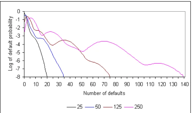
An important feature of the default probability distribution is its long tail. To get a better understanding of the distribution along the tail, a logarithmic plot is presented in Figure 2. It exhibits an unusual bumpy distribution that has a direct impact on the prices of the non-equity tranches. Such bumpy tail distributions have also been encountered by other researchers in the field before. The bumpy feature appears to be more pronounced for smaller maturities. As can be noted from Figure 3, it is also dependent on the number of credit names, becoming visible for a few tens or so credit names and getting more bumpy as their number increases. These characteristics can be analytically understood as in Appendix C.
with the economy and the second one with the industry. The implied parameters are consistent with this interpretation. The first factor name couples more strongly to the credit names compared to the second factor name, at the same time being less likely to generate default causing events. The implied default correlations turn out to be somewhat larger compared to the historical default correlations as expected in a risk neutral world.
3
Markov Chain Formulation
There is another approach to the model that has the potential to be useful for further development. Our approach so far could be termed static as it involves working with the joint survival probability distribution describing the default environment for all times. It turns out that there is an alternate formulation that could be termed dynamic being capable of accommodating additional features such as stochasticity of parameters. Let x(t) be a column vector representing the state of the system at time t, evolving according to
dxT(t)
dt =−x
T(t)G(t), (21)
where a superscriptT denotes transpose and the matrix −G(t) is the generator of this continuous time Markov chain3. The entries ofx(t) are the probabilities that the system will be found in their associated states at timet. Because these probabilities should add up to one, we requirexT(t)v = 1
where v is a column vector containing ones for all its entries. Besides, these probabilities should remain non-negative at all times. These requirements are ensured by the constraintsG(t)v = 0 and that the diagonal elements ofG(t) are non-negative and the off-diagonal elements non-positive. The above linear system could in general involve a time-dependent G(t), but we would be concerned with time-independence, or utmost a time dependence such thatG(t)’s commute among themselves for different t’s, that isG(s)G(t) =G(t)G(s) for any two times sand t. Then (21) solves to
xT(t) =xT(0)e−
Rt
0dsG(s), (22)
where the column vector x(0), representing the state of the system at time zero, contains the probabilities that the system starts off in various states.
To start with, consider a two-state system for one credit name with u = (1,0)T representing the undefaulted and d= (0,1)T representing the defaulted states, and with
G(t) =λ(t)A, A= 1 −1
0 0
!
. (23)
Note that v is a right eigenvector of A with zero eigenvalue. Another right eigenvector is u with eigenvalue one. If we are interested in the probability that the system is in the defaulted state d
at timet, we can expressdin terms of v andu asd=v−u to determine that probability,
xT(t)d=xT(0)e−
Rt
0dsλ(s)A(v−u) =xT(0)
v−e−
Rt
0dsλ(s)u
= 1−e−
Rt
0dsλ(s)xT(0)u. (24)
That is, if the credit name started off at time zero in the undefaulted state withx(0) =u, it would end up in the defaulted state at time twith probability 1−exp−Rt
0dsλ(s)
.
3Markov chains have been used in credit risk modeling. See Jarrow, Lando and Turnbull [1997] and more recently
This approach can be extended to a collection of ncredit names, the state space of which is a tensor product of individual state spaces spanned by
⊗ni=1(ui ordi), (25)
whereui anddi represent respectively the ith individual undefaulted and defaulted states. For the vector v in the collective state space with ones for all its entries, we have v =⊗ni=1vi. Motivated by our results in the previous sections, in particular equation (11), we set
G(t) =
n
X
i=1
λi(t)Ai+ m
X
r=1
ζr(t)
"
1−
n
Y
i=1
(1−γir(t)Ai)
#
. (26)
HereAi acts asA on theithindividual state space and as identity on all others. It is easily checked
thatG(t)v= 0. For the parameter constraints discussed earlier, it can be verified that the diagonal and the off-diagonal requirements onG(t) are also satisfied. Eigenvalues ofG(t) are given byπij...(t) as expressed in (11) with the right eigenvector as a tensor product of u’s for each of the names in the list{i, j, ...}and v’s for the rest of the names. The probability that credit names, say 1,2, ..., ν, are in the defaulted state at timet and the rest are not is given by
xT(t) [⊗νr=1dr]
⊗nr=ν+1ur
=xT(0)e−R
t
0dsG(s)[⊗νr=1(vr−ur)]⊗nr=ν+1ur. (27)
This can be evaluated by expanding the product containing (v−u)’s. Because each state vector in the expansion is a right eigenvector ofG(t), the result is a sum of exponentials. For a collection with all the names starting off as undefaulted, this result agrees with our earlier result of equation (5). For a homogeneous collection of credit names, one finds for this probability
P[ν] =
ν
X
r=0
(−1)r(νr)pn−ν+rQ[ν−r], (28)
whereP andQare as defined earlier, but with only the number of names as subscripts. Each credit name is assumed to have started off at time zero in the undefaulted state with probability p. For
p = 1, this result agrees with equation (7). When concerned with only the number of defaults, it should be multiplied by the number of combinations ofν out of ncredit names.
To appreciate the usefulness of this approach, let us allow for some probability that the defaulted state can recover to become undefaulted, with
A= 1−ǫ −1 +ǫ
−ǫ ǫ
!
. (29)
Note that v is still a right eigenvector of A with eigenvalue zero. The other right eigenvector is
w= (1−ǫ,−ǫ)T with eigenvalue one. In terms of these,u and dcan be expressed as
u=ǫv+w, d= (1−ǫ)v−w. (30)
For the probability that given ν names in a homogeneous collection are in the defaulted state at timet and the rest are not, we find
P[ν]=
ν
X
r=0
n−ν
X
s=0
(−1)r(νr) n−sν
where again each credit name is assumed to have started off at time zero in the undefaulted state with probabilityp. It is not straightforward to obtain this result from our earlier approach.
Given a homogeneous collection at time twithν names defaulted, the probability of additional
knames defaulting during (t, t+dt) is
"
1−(n−ν)λdt− m
X
r=1
ζrdt
#
δk0+
h
(n−ν)λdtiδk1+
n−ν
k
Xm
r=1
ζrγrk(1−γr)n−ν−kdt, (32)
where 0≤k≤n−ν and the parameters could in general be time dependent. This perhaps obvious result can be obtained from a Markov chain representation of the model discussed above. These transition probabilities, from ν defaults at time t toν+k defaults at time t+dt, can be used to simulate default paths from time zero onwards. Average of prices computed for these default paths gives the desired price as an alternative to the sem-analytical approach. One can also derive an evolution equation for the joint default probability from these transition probabilities,
dP{ν}
dt =−
"
(n−ν)λ+
m
X
r=1
ζr
#
P{ν}+ (n−ν+ 1)λP{ν−1}+
m
X
r=1
ζr(1−γr)n−ν
ν
X
k=0
n−ν+k
k
γrkP{ν−k},
(33) where P{ν} is the probability that ν names are in the defaulted state at time t summed over all
combinations of ν out of n credit names. This equation is also in the form of a continuous time Markov chain as can easily be verified.
For a general collection of credit names, a recursion relation can be derived from the expression forG(t) to obtain the probability that any ν credit names are in the defaulted state at timet and the rest are not. Considering the cases where, say, thenth credit name is in the unordn=vn−un
states, we get
P{ν,n}(λ, ζ) =P{ν−1,n−1}(λ, ζ) +e−
Rt
0dsλn(s)
h
P{ν,n−1}(λ, ζ′)−P{ν−1,n−1}(λ, ζ′)
i
, (34)
where a subscript {ν, n} denotes sum of all combinations of ν out of n credit names, λn in the exponential is to be expressed in terms ofλn andζr’s, and
ζr′ =ζr(1−γnr). (35)
The recursion relation can be used to update the default probability distribution recursively, adding the credit names one by one to the collection. With the appropriate boundary conditions, for instance P{0,0} = 1, P{ν,n} = 0 for ν < 0 and ν > n, and continuing through the recursion, all
the credit names can be taken care of to yield the desired probability. These recursive procedures are computationally intensive and are expected to be useful for a small number of credit names, or when a few hazard rates are either all smaller or larger in an otherwise homogeneous collection of credit names.
4
Instantaneous Correlation Matrix
The model in general contains a large number of parameters. They are however necessary to account for a rich structure of default correlations. Note that equation (12) for ρij(t) specifies
only off-diagonal elements to a matrix of correlations. To make it complete, one could introduce diagonal elementsρi(t) by
ρi(t)λi(t) =
m
X
r=1
γir(t)2ζr(t). (36)
Together with ρij(t)
q
λi(t)λj(t)’s, these form a symmetric matrix Σ, referred to in the following
as the correlation matrix. An n×m matrix Γ can be formed with Γir(t) = γir(t)pζr(t), so that
we can write (12) in matrix notation as Σ = ΓΓT where a superscript T denotes transpose. Thus, given a general set of γ and ζ parameters, Σ is of rank m or n whichever is smaller. In order to generate correlations that can form a matrix of rank not less thanr, one would need a multi-factor model with at least as many factors asr. The equation Σ = ΓΓT relates a subset of the parameters to Σ. Others play a role in higher order correlations.
The matrix relation Σ = ΓΓT implies that the model generates an instantaneous correlation
matrix that is completely positive. A completely positive matrix is one that can be decomposed as ΓΓT where Γ is (entry-wise) non-negative. Consequently, it is both positive semidefinite and
non-negative (called doubly non-negative). Characterizing a given matrix so that it is completely positive is an open problem in matrix theory. It is known however that diagonal dominance is sufficient for a non-negative symmetric matrix to become completely positive. Thus, an instanta-neous correlation matrix, if supplied, can be diagonally completed to become completely positive. But not all diagonally completed completely positive Σ’s are acceptable to the model as correlation matrices. In order that the impliedλ(t)’s can be non-negative, the matrix Γ should obey
m
X
r=1
Γir(t)Maxk(Γkr(t)) = m
X
r=1
γir(t)ζr(t)Maxk(γkr(t))≤ m
X
r=1
γir(t)ζr(t)≤λi(t), (37)
where, for each r, Maxk(Γkr) is the largest of Γkr, k = 1, ..., n. Because a non-negative Γ solving
Σ = ΓΓT is in general not unique, Γ itself should be made available to the model when Σ is supplied. Instantaneous correlations are subject to certain constraints as a consequence of (37) besides being part of a completely positive matrix. One of them is an upper bound on ρij inferred earlier from the requirement on the conditional two-point joint default probability density, pij ≤ λi. In general, the requirement on a higher order conditional joint default probability density is pijk...≤ pij... where the later list{i, j, ...}is a subset of the former{i, j, k, ..}. Analogous requirement holds for the dual density, πijk... ≥ πij..., since having another name in the list can not decrease the probability of at least one name defaulting. For three-point joint defaults, πijk≥πij implies
pij ≥ pijk≥pik+pjk−pk,
or pi+pj −2pij ≤ (pi+pk−2pik) + (pj+pk−2pjk). (38)
This is the triangle inequality for a distance measuredij between namesiand j given by
dij =pi+pj−2pij =λi+λj−2ρijqλiλj. (39)
values from zero to qλi/λj whenλi≤λj,dij takes values from|λi−λj|toλi+λj. This distance
measure is also derivable from (37) because of
Σik+ Σjk−Σij = m
X
r=1
[gkr−girgjr(1−gkr)−(1−gir)(1−gjr)gkr]zr≤ m
X
r=1
gkrzr, (40)
where zr = (Maxk(Γkr))2 and gir = Γir/√zr ≤ 1. Using (37) and identifying Σij with pij, this
relation can be rearranged to obtain the triangle inequality.
The distance measure (39) is a special case of a distance measurePA+PB−2PAB between two
binomial events A and B where PA and PB are probabilities of A and B respectively and PAB is their joint probability. We could define other distance measures for credit names making use of, for instance, default probability densities of iand j given that some other names have defaulted. A distance measure that has the familiar look is the distance between two “vectors” of lengths√λi
and p
λj withρij as the cosine of the angle between them. This is the square root of dij that does satisfy the triangle inequality because ofdij but the triangle inequality fordij is stronger. However,
dij is not a good distance measure for determining a correlated neighborhood to a credit name when there are significant variations in the hazard rates, since it is not just the correlations that define it but the hazard rates as well.
5
A Scaled Correlation Model
A simple generalization of the homogeneous model to heterogeneity is to allow for non-uniform haz-ard rates but to keep theγ parameters uniform accross all credit names, so that the instantaneous default correlations are
ρij(t) = q 1
λi(t)λj(t) m
X
r=1
γr(t)2ζr(t). (41)
These form part of a rank one matrix. However, in this framework,ρij can not reach its upper bound discussed earlier unless one of the names i or j has the lowest hazard rate. Hence this approach could run into trouble for collections with widely varying hazard rates and relatively large default correlations. A maximally correlated collection of credit names could be the limiting case of a suitably defined uniform correlation structure, but one would need n factor names to model even such a simple setup because differing hazard rates would result in a correlation matrix of rank n. An upper bound on the correlations suggests a coupling of the two aspects of heterogeneity, namely, non-uniform hazard rates and a non-uniform structure of default correlations. Let us discuss here one possible approach addressing the issue of non-uniform hazard rates by decoupling them from the correlations. This could be applicable, for instance, to collection of directly dependent credit names forming a chain of supplier-consumer dependency. With the credit names ordered according toλ1(t)≤λ2(t)...≤λn(t), let us rewrite the correlations as
ρij(t)qλi(t)λj(t) =λi(t)ρ′ij(t), i < j, (42)
so that the scaled correlations ρ′
ij(t) can take values from zero to one. Now considern×m factor
names, a cross product of two sets, the first responsible for the hazard rate structure and the second for the correlations. Witha= 1, ..., nand r = 1, ..., mtogether labeling the factor names, let
γir(t)→ γiar(t) =γir(t) fora≤i, 0 fora > i,
with λ0(t) = 0. This makes ζ’s “dimensionless”. In this setup, the equations for the first two conditional probability densities read
λi(t) = λi(t) +λi(t)
m
X
r=1
γir(t)ζr(t),
ρ′ij(t) =
m
X
r=1
γir(t)γjr(t)ζr(t). (44)
Hazard rates are now decoupled from the scaled correlations as expected. For the higher order conditional probability densities, we get
pij...(t) =λi(t)
m
X
r=1
(γir(t)γjr(t)...)ζr(t), i <{j, ...}. (45)
The π-densities in equation (11) can now be expressed as
πij...(t) =X
k
λk(t) +λk(t)
m
X
r=1
γkr(t)ζr(t)Y
l>k
(1−γlr(t))
, (46)
where k and l run over only those credit names that are in the subscripted list {i, j, ...}. Thus, out of then×m factor names,nof the component factors are now “forgotten” and the model has become what may be simply called a m-factor model.
For a homogeneous collection of credit names, this formalism reduces to the homogeneous model discussed in section 2. It can now be used to model non-uniform hazard rates with a “uniform” correlation structure, that is, a uniform structure of scaled correlations. Dropping the subscripts for the credit names for all the parameters, except for the hazard rates, one obtains expressions looking very similar to those for the homogeneous names. Parameterization could be done along the same lines as in equations (18) or (20) for homogeneous names. The approach however is computationally slow while computing Pij...’s in (5) where one needs to keep track of all combinations of credit
names. Recursive approach discussed below, though still computationally intensive, could be a better alternative.
Our remarks of the previous section on the correlation matrix Σ are applicable to the scaled correlation matrix Σ′ as well. That is, a scaled correlation matrix, if supplied, should be completely positive with the matrix Γ′ obeying
m
X
r=1
Γ′ir(t)Maxk(Γ′kr(t))≤1. (47)
When these hold, it can be shown along steps similar to (43) that there exists a Γ satisfying (37), yielding a completely positive correlation matrix Σ = ΓΓT. When the system admits a decoupling
of the hazard rates from the correlations as discussed above, we can also deduce from (47) a stronger distance measure d′ij = 1−ρ′ij (that impliesdij of equation (39)) based on just the scaled correlations, perhaps a better candidate for determining correlated neighborhoods.
In this model, the expression for G(t) of the Markov chain formulation is
G(t) =
n
X
i=1
λi(t)Ai+λi(t)Ai
m
X
r=1
γir(t)ζr(t)
n
Y
j=i+1
(1−γjr(t)Aj)
where again the credit names are ordered according toλ1(t)≤λ2(t)≤...λn(t). Eigenvalues ofG(t)
are given by πij...(t) as expressed in (46) with the right eigenvector as a tensor product of u’s for each of the names in the list {i, j, ...} and v’s for the rest of the names. Recursion relation (34), that has been derived for a generalG(t), can be used to update the default probability distribution, but in terms of our original γ and ζ parameters. For a “uniform” correlation structure discussed above, it can be used in terms of our newγ and ζ parameters with
ζr′ =ζr 1−γr
1−Pm
s=1γs2ζs
. (49)
Here the default probability distribution is updated by adding to the collection a credit name with the next largest hazard rate. Analogous, but less convenient, recursion relations can be derived for adding credit names with the next smallest hazard rates or for the case of non-uniform scaled correlation structures.
6
Conclusion
In this article, a semi-analytical parametric model for dependent defaults is presented. It is based on instantaneous default correlation and is hence capable of handling a term structure of default correlations that could be helpful in accommodating a series of instruments of increasing maturities into a single framework. It involves a probability parameter representing higher order correlations that could explain clustering tendency of credit defaults known as default contagion. It admits a formulation in terms of a continuous time Markov chain that could be useful for incorporating additional dynamical features such as stochasticity of model parameters.
It is a multi-factor model but multiplicity of factors does not introduce major complexities. A two factor model with four free parameters and a constant hazard rate is used to provide perfect fits to the four non-equity tranches of CDX.NA.IG and iTraxx Europe CDOs of 5, 7 and 10 year maturities. Allowing for log-linear time dependence for the hazard rate enables us to obtain perfect fits to all the five tranches of both CDX.NA.IG and iTraxx Europe CDOs for all three maturities. These fits could be useful for pricing non-standard products and performing sensitivity analysis for hedging purposes.
The model is based on the assumption of conditional independence of defaults at differing times. That is, if a credit name has survived an instant, an event at that instant does not have any further influence on the credit name. This ignores response times to events causing defaults and the model as such is expected to be applicable at relatively larger time scales. The unrealistic implication that all defaults associated with an event would occur instantaneously could be addressed by introducing time delays in responding to events. This issue will be discussed elsewhere.
A
Expression for Joint Survival Probability
Here, let us derive expression (2) for the joint survival probability Q(t1, ..., tn). As discussed in the article, let us assume that defaults at differing times are conditionally independent. In other words, given that credit names i and j have survived up to times ti and tj respectively, ti 6= tj, their respective defaults at ti and tj are independent of each other. This means
Q−1(ti, tj)∂ 2Q(t
i, tj)
∂ti∂tj dtidtj =
−Q−1(ti, tj)∂Q(ti, tj)
∂ti dti
"
−Q−1(ti, tj)∂Q(ti, tj)
∂tj dtj
#
, (50)
where we have shown only the dependence onti and tj for simplicity. Rearranging the terms,
∂Q(ti, tj)
∂ti
−1"∂2Q(ti, tj)
∂ti∂tj
#
=Q−1(ti, tj)
"
∂Q(ti, tj)
∂tj
#
. (51)
This can be simplified to read
∂ ∂tjLn
−∂Q(∂titi, tj)
= ∂
∂tjLnQ(ti, tj). (52)
Further simplification leads to
∂ ∂tjLn
− ∂
∂tiLnQ(ti, tj)
= 0. (53)
This implies, for ordered times, as long as time ordering is maintained, that−∂LnQ/∂t(i) is inde-pendent of t(j) for allj 6=i. With all the t(j)’s reaching t(i) in the limit, it becomes a function of
t(i) only. It is in fact the probability density that credit name (i) defaults at t(i), given that names (i+ 1)...have not defaulted at t(i) while names (1)...(i−1) are not looked at (considering models where it is independent of the ordering among names not defaulted, or not looked at). In terms of
πij...(t)’s introduced in (2), we may write
∂ ∂t(i)
LnQ(t(1)...) =−π(i)...(n)(t(i))−π(i+1)...(n)(t(i))
. (54)
To see this, note that 1−π(i+1)...(t)dt is the conditional probability that none of the credit names
(i+ 1)... default during the interval (t, t+dt) (names (1)...(i) are not looked at). It exceeds 1−π(i)...(t)dt (here, names (1)...(i−1) are not looked at) by exactly the probability density that
credit name (i) defaults at t, given that names (i+ 1)...have not defaulted. Let us first integrate the above fori= 1 from time zero to t(1). We do not encounter othert(i)’s during this sincet(1) is the smallest of the ordered times. We get
LnQ(t(1)...) = LnQ(1)(t(2)...)−
Z t(1)
0 ds π(1)...(n)(s) +
Z t(1)
0 ds π(2)...(n)(s), (55) where Q(1) is obtained from Q by settingt(1) = 0. Equation (54) holds for Q(1) as well, because, fori≥2, its right hand side is independent of t(1) and we can sett(1) = 0 in Q. Integrating it for
i= 2 from time zero to t(2), we get an expression forQ(1) as an integral up tot(2),
LnQ(1)(t(2)...) = LnQ(1)(2)(t(3)...)−
Z t(2)
0
ds π(2)...(n)(s) +
Z t(2)
0
ds π(3)...(n)(s), (56)
whereQ(1)(2) has both t(1) and t(2) set to zero. Combining the two equations, we get
LnQ(t(1)...) = LnQ(1)(2)(t(3)...)−
Z t(1)
0 ds π(1)...(n)(s)−
Z t(2)
t(1)
ds π(2)...(n)(s) +
Z t(2)
B
Expressions for Homogeneous Pricing
Here, let us derive some simplified results for homogeneous names useful in the computation. For aνthto default premium leg, the probability that less than ν names have defaulted beforetcan be obtained from (7). Keeping only the number of names as subscripts, it reads
ν−1
X
r=0
(nr)P[r] =
ν−1
X
r=0 (nr)
r
X
s=0
(−1)s(rs)Q[r−s]=
ν−1
X
r=0
(nr)CνrQ[r],
where Cνr =
ν−1−r
X
s=0
(−1)s n−sr
. (58)
For the default leg, we need the probability that less thanν names have defaulted beforetand the number of defaults during (t, t+dt) makes it ν or more. This is obtained by differentiating the above with respect to time. The results are a weighted sum of exponentials. For unit notional per name, uniform constant recovery rate R, and spread premium s, the legs can be computed as a sum of one-name CDS expressions,
Default Leg = (1−R)
ν−1
X
r=0
(nr)CνrDπ[n−r]
,
Premium Leg = s ν−1
X
r=0
(nr)CνrPπ[n−r]
, (59)
where, for constant model parameters, constant interest rate r, time to maturity T and uniform period lengthsδ, the one-name CDS expressions are
D(λ) = λ
λ+r
h
1−e−(λ+r)Ti, P(λ) =δ
1 +λδ
2
1
−e−(λ+r)T
e(λ+r)δ−1 . (60)
Next consider a CDO tranche. Under the homogeneous setting with uniform notionals and a uniform constant recovery rate, we can determineνLandνH, the number of defaults corresponding to the attachment and detachment points of the tranche respectively, the next closest integers if they turn out to fractional. Then the legs can be computed as a sum ofνthto default legs,
Default Leg =
νH
X
ν=νL
wν
νthto Default Leg, (61)
wherewν = 1, except perhaps forν =νLorνH where it could be a fractionwνL orwνH respectively. Substituting for theνthto default leg and simplifying,
Default Leg = (1−R)
νH−1
X
r=0
(nr)Cr′Dπ[n−r]
,
Premium Leg = s(1−R)
νH−1
X
r=0
(nr)Cr′P
π[n−r]
,
where Cr′ =
νH
X
ν=Max(νL,r+1)
wνCνr. (62)
C
Structure of the Default Distribution
Here, let us try to undertsand the structure of the joint default probability distribution, in partic-ular the bumps visible on its long tail. The probability of finding ν defaults over time T in the homogeneous case with constant parameters can be expressed as
P{ν} = (nν) ν
X
k=0
(−1)k(νk)Q[ν−k]= (nν) ν
X
k=0
(−1)k(νk) exp−π[n−ν+k]T
= (nν)
ν
X
k=0
(−1)k(νk) exp
(
−(n−ν+k)λT − m
X
r=1
ζrTh1−(1−γr)n−ν+ki
)
= (nν)
ν
X
k=0
(−1)k(νk)e−λTn−ν+k m
Y
r=1
e−ζrTexphζrT(1−γr)n−ν+ki
= (nν) ν
X
k=0
(−1)k(νk)
e−λTn−ν+k
∞
X
i1...im=0
m
Y
r=1
e−ζrT(ζrT)
ir
ir!
h
(1−γr)irin−ν+k
=
∞
X
i1...im=0
m
Y
r=1
"
e−ζrT(ζrT)
ir
ir!
#
(nν)
"
e−λT m
Y
r=1
(1−γr)ir
#n−ν"
1−e−λT m
Y
r=1
(1−γr)ir
#ν
.
(63)
This is a mixture of binomial distributions. This result can also be inferred from our assumption of conditional independence of defaults given the factor states, by writing it down as binomial dis-tributions conditional on the arrival of a number of events generated by the factor names, summed over the Poisson distributed probabilities of arrival of those events. The binomial distributions are positioned at
νi ≈n
"
1−e−λT m
Y
r=1
(1−γr)ir
#
(64)
with the mixing weights
wi= m
Y
r=1
"
e−ζrT(ζrT)
ir
ir!
#
. (65)
These contribute to the bumps in our joint default probability distribution. The width of the bumps are ≈ 2σi where σi = p
νi(n−νi)/n, that increases with νi for νi < n/2. The peaks are
≈wi/√2πσi. The width increases only as √n with n, making the bumps more pronounced as n
increases. For very large n, one could approximate the joint default probability distribution as a set of weights concentrated at the above positions.
In a two-factor model with γ1> γ2, the positions of the bumps as a fraction of nare
1−e−λT, 1−e−λT(1−γ2), ... 1−e−λT(1−γ2)i2, 1−e−λT(1−γ1), ... (66)
The first bump is due toλ. It is followed byγ2−bumps due to the second factor name. The number ofγ2−bumps before we encounter aγ1−bump due to the first factor name is given by the largesti2 such that (1−γ2)i2 >1−γ1. As an example, ifγ
D
Arbitrary Precision Code for CDO Pricing
The code below is written for a simple to use, but a powerful, arbitrary precision calculator available from “http://directory.fsf.org/calc.html”. On copying into a file, say “cdo.txt”, and running the command “calc -f cdo.txt”, it prints out iTraxx Europe 5-year CDO tranche premiums.
m = 2; n = 125; R = 0.40;
T = 5; ir = 0.035; dc = 0.25; dt = 1.0; mat tra[] = {0.0,0.03,0.06,0.09,0.12,0.22}; mat gam[m]; mat zta[m]; mat tht[m];
rho = 1.862/100; gam[0] = 26.150/100; if (m > 1) gam[1] = 7.047/100;
tht[0] = 39.606*pi()/180;
lam0 = 29.2121/10000; mulam = 0.25985; for (r = 0; r < m; r++) {
tmp = (r<m-1)? power(cos(tht[r]),2) : 1.0;
for (s = 0; s < r; s++) tmp *= power(sin(tht[s]),2); zta[r] = tmp*rho/(gam[r]*gam[r]);
}
expmu = exp(mulam*dt);
ntraL = 0; ntraH = 4; eps = epsilon(1.0e-10);
for (ntra = 0; ntra < ntraL; ntra++) epsilon(epsilon()*1e-10); for (ntra = ntraL; ntra <= ntraH; ntra++) {
dleg = pleg = 0.0; epsilon(epsilon()*1e-10); atL = n*tra[ntra]/(1-R); nuL = ceil(atL+eps); atH = n*tra[ntra+1]/(1-R); nuH = ceil(atH-eps); for (r = 0; r < nuH; r++) {
cprr = 0; nufr = (r < nuL)? nuL : r+1; for (nu = nufr; nu <= nuH; nu++) {
cnur = 0; sign = 1;
for (s = 0; s < nu-r; s++) { cnur += sign*comb(n-r,s); sign *= -1; } cprr += cnur*((nu<atL+1)?(nu-atL):(nu>atH)?(atH-nu+1):1);
}
mult = comb(n,r)*cprr;
for(pinr = n-r, s = 0; s < m; s++)
pinr += zta[s]*(1.0-(n-r)*gam[s]-power(1.0-gam[s],n-r)); for (pinr *= lam0, t = 0.0; t < T-eps; t += dt) {
temp = exp(-(pinr+ir)*dt);
dleg += mult*(1.0-temp)*(pinr/(pinr+ir));
pleg += mult*(1.0-temp)*dc*(1.0+0.5*pinr*dc)/(exp((pinr+ir)*dc)-1.0); mult *= temp; pinr *= expmu;
} }
premium = (atL<eps)? 100*(dleg-0.05*pleg)/atH : 10000*dleg/pleg;
References
[1] Albanese, C., O. Chen and A. DAlessandro (2005), “Dynamic Credit Correlation Modeling”, Working paper, http://defaultrisk.com/pp corr 80.htm.
[2] Albanese, C., G. Campolieti, O. Chen and A. Zavidonov (2003), Credit Barrier Models, Risk 16 (6), pp. 109-113.
[3] Andersen, L., J. Sidenius and S. Basu (2003), All Your Hedges in One Basket, Risk, November, pp. 67 - 72.
[4] Arvanitis, A. and J. Gregory (2001), “Credit: The Complete Guide to Pricing, Hedging and Risk Management”, Risk Publications.
[5] Avellaneda, M. and J. Zhu (2001), Distance to Default, Risk 14 (12), pp. 125-129.
[6] Baxter, M. (2006), “Levy Process Dynamic Modeling of Single-Name Credits and CDO Tranches”, Working paper, http://defaultrisk.com/pp crdrv 110.htm.
[7] Bennani, N. (2005), “The Forward Loss Model: A Dynamic Term Structure Approach for the Pricing of Portfolio Credit Derivatives”, Working paper, http://defaultrisk.com/ pp crdrv 95.htm.
[8] Berman, A. and N. Shaked-Monderer (2003), “Completely Positive Matrices”, World Scientific, New Jersey.
[9] Brigo, D., A. Pallavicini and R. Torresetti (2006), “Calibration of CDO Tranches with the Dynamical Generalized-Poisson Loss Model”, Working paper, http://www.defaultrisk.com/ pp crdrv117.htm.
[10] Chapovsky, A., A. Rennie and P. A. C. Tavares (2006), “Stochastic Intensity Modeling for Structured Credit Exotics”, Working paper, http://defaultrisk.com/pp crdrv 136.htm.
[11] Das, S. R., D. Duffie and N. Kapadia (2005), “Common Failings: How Corporate Defaults are Correlated”, Working Paper, Santa Clara University, February, 2005.
[12] Davis, M. and L. Violet (2000), “Modeling Default Correlation in Bond Portfolios”, Working paper, Imperial College, London, 2000.
[13] Di Graziano, G. and C. Rogers (2005), “A Dynamic Approach to the Modeling of Correla-tion Credit Derivatives Using Markov Chains”, Working paper, http://www.defaultrisk.com/ pp crdrv 88.htm.
[14] Duffie, D. and N. Garleanu (2001), “Risk and the Valuation of Collateralized Debt Obliga-tions”, Financial Analysts Journal, 57, pp. 41-59.
[15] Duffie, D. and K. Singleton (1999), “Modeling Term Structures of Defaultable Bonds”, Review of Financial Studies, 12, pp. 687-720.
[16] Elouerkhaoui, Y. (2003), “Pricing and Hedging in a Dynamic Credit Model”, Citigroup Work-ing paper.
[18] Finger, C. C. (2004), “Issues in the Pricing of Synthetic CDOs”, The Journal of Credit Risk, 1(1): pp. 113-124.
[19] Friend, A. and E. Rogge (2004), Correlation at First Sight, Working Paper, ABN AMRO.
[20] Gregory, J. and J.P. Laurent (2004), In the Core of Correlation, Risk, October, pp. 87-91.
[21] Giesecke, K. (2001), “Correlated Default with Incomplete Information”, Journal of Banking and Finance, Humboldt Universitat Berlin, October 2001.
[22] Hager, S. and R. Sch¨obel (2005), A Note on the Correlation Smile, Tbinger Diskussionsbeitrag 297.
[23] Hull, J and A. White (2006), “Valuing Credit Derivatives Using an Implied Copula Approach”, Working Paper, Joseph L. Rotman School of Management, May 2006.
[24] Jarrow, R. and F. Yu (2000), “Counterparty Risk and the Pricing of Defaultable Securities”, Journal of Finance, 56, pp. 1765-1799.
[25] Jarrow, R., D. Lando and S. M. Turnbull (1997), “A Markov Model for the Term Structure of Credit Risk Spreads”, Review of Financial Studies 10, pp. 481-523.
[26] Joshi, M. and A. Stacey (2005), “Intensity Gamma: A New Approach to Pricing Credit Derivatives”.
[27] Li, D. X. (2000), On Default Correlation: a Copula Function Approach, The Journal of Fixed Income, Vol. 9, March, pp. 43-54.
[28] Lindskog, F. and A. McNeil (2003), “Common Poisson Shock Models: Applications to Insur-ance and Credit Risk Modeling”, ASTIN Bulletin, 33(2), pp. 209-238.
[29] Marshall, A. and I. Olkin (1967), “A Multivariate Exponential Distribution”, Journal of the American Statistical Association, 62, 30-44.
[30] Mashal, R., M. Naldi and G. Tejwani (2004), The Implications of Implied Correlation, Lehman Brothers, Quantitative Credit Research, Working Paper.
[31] McGinty, L., E. Beinstein, R. Ahluwalia and M. Watts (2004), Introducing Base Correlations, Credit Derivatives Strategy, JP Morgan, March 2004.
[32] OKane, D. and L. Schl¨ogl (2003), The Large Homogeneous Portfolio Approximation with the Student-t Copula, Working Paper, Lehman Brothers International, July 2003.
[33] Schmidt, W. and I. Ward (2002), Pricing Default Baskets, Risk 15 (1), pp. 111-114.
[34] Sch¨onbucher, P. (2003), “Information Driven Default Contagion”, Working paper, D-MATH, ETH Z¨urich, December 2003.
[35] Sch¨onbucher, P. (2005), “Portfolio Losses and the Term Structure of Loss Transition Rates: A New Methodology for the Pricing of Portfolio Credit Derivatives”, Working paper, http://defaultrisk.com/pp model 74.htm.
[37] Sidenius, J., V. Piterbarg and L. Andersen (2005), “A New Framework for Dynamic Credit Portfolio Loss Modeling”, Working paper, http://defaultrisk.com/pp model 83.htm.
[image:22.612.121.490.240.465.2][38] Vasicek, O. (1987), Probability of Loss on Loan Portfolio, Working Paper, KMV Corporation.
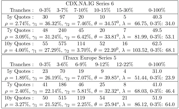
Table 1: Two-factor perfect fits to the four non-equity tranches of CDX.NA.IG and iTraxx Europe CDOs for the market quotes on June 2, 2006 computed in the semi-analytical approach assuming a constant hazard rate. There are 125 names with a uniform recovery rate of 40%. Premiums are paid quarterly. Interest rate is assumed at a constant 5% for CDX.NA.IG and 3.5% for iTraxx Europe CDOs. Equity tranche is quoted as an upfront fee in percent (plus 500bp per year running) and the other tranches are quoted as spreads per year in bp.
CDX.NA.IG Series 6
Tranches : 0-3% 3-7% 7-10% 10-15% 15-30% 0-100% 5y Quotes : 30 97 20 10 5 40.3
ρ = 2.74%, γ1 = 36.32%,γ2 = 7.46%, θ = 34.570,λ= 66.75, 0-3%: 34.0 7y Quotes : 48 240 45 20 7 49.5
ρ = 3.09%, γ1 = 31.24%,γ2 = 6.42%, θ = 33.810,λ= 81.99, 0-3%: 53.1 10y Quotes : 55 575 114 52 16 62.5
ρ = 4.00%, γ1 = 27.29%,γ2 = 3.70%, θ= 22.200,λ= 103.52, 0-3%: 68.1 iTraxx Europe Series 5
Tranches : 0-3% 3-6% 6-9% 9-12% 12-22% 0-100%
5y Quotes : 23 70 19 9 4 31.0
ρ = 1.89%, γ1 = 26.19%,γ2 = 7.07%, θ = 39.85o,λ= 51.44, 0-3%: 23.9 7y Quotes : 41 186 46 25 8 41.0
ρ = 2.40%, γ1 = 22.14%,γ2 = 5.81%, θ = 32.32o,λ= 68.03, 0-3%: 46.4 10y Quotes : 50 515 119 54 21 51.9
Table 2: Two-factor perfect fits to all the five tranches of CDX.NA.IG and iTraxx Europe CDOs for the market quotes on June 2, 2006 computed in the semi-analytical approach assuming a log-linear time dependence for the hazard rate. There are 125 names with a uniform recovery rate of 40%. Premiums are paid quarterly. Interest rate is assumed at a constant 5% for CDX.NA.IG and 3.5% for iTraxx Europe CDOs. Equity tranche is quoted as an upfront fee in percent (plus 500bp per year running) and the other tranches are quoted as spreads per year in bp.
CDX.NA.IG Series 6
Tranches : 0-3% 3-7% 7-10% 10-15% 15-30% 0-100% 5y Quotes : 30 97 20 10 5 40.3
ρ = 2.47%, γ1 = 35.95%,γ2 = 7.64%,θ = 31.260,λ(0) = 0.012, κλ = 2.560
7y Quotes : 48 240 45 20 7 49.5
ρ = 3.30%, γ1 = 52.84%,γ2 = 14.08%, θ= 33.870,λ(0) = 13.34, κλ = 0.491
10y Quotes : 55 575 114 52 16 62.5
ρ = 7.09%, γ1 = 65.72%,γ2 = 14.21%, θ= 25.330,λ(0) = 30.23, κλ = 0.246 iTraxx Europe Series 5
Tranches : 0-3% 3-6% 6-9% 9-12% 12-22% 0-100%
5y Quotes : 23 70 19 9 4 31.0
ρ = 1.86%, γ1 = 26.15%,γ2 = 7.05%,θ = 39.61o,λ(0) = 29.21, κλ = 0.260
7y Quotes : 41 186 46 25 8 41.0
ρ = 2.08%, γ1 = 22.52%,γ2 = 8.87%, θ= 30.25o,λ(0) = 5.52,κλ = 0.633
10y Quotes : 50 515 119 54 21 51.9
[image:23.612.145.470.508.699.2]ρ= 4.58%, γ1 = 41.79%, γ2 = 10.65%,θ= 27.79o,λ(0) = 12.46, κλ = 0.351
Figure 2: Logarithmic plot of the joint default probability distributions over 5, 7 and 10 years for 125 credit names for the model parameters from Table 2 calibrated to iTraxx Europe CDOs of corresponding maturities.
[image:24.612.144.470.487.679.2]