A Simple Algorithm for Generating Stable Biped Walking Patterns

A Simple Algorithm for Generating Stable Biped Walking

Patterns

Hayder F. N.

Al-Shuka

Baghdad University,Mech. Eng.

Dep., Iraq

Burkhard J.

Corves

RWTH Aachen University, IGM,

Germany

Wen Hong Zhu

Canadian Space Agency, Canada

Bram

Vanderborght

Department of Mechanical Engineering, Vrije Universiteit

Brussel, Belgium

ABSTRACT

This paper proposes a thorough algorithm that can tune the walking parameters (hip height, distance traveled by the hip, and times of single support phase SSP and double support phase DSP) to satisfy the kinematic and dynamic constraints: singularity condition at the knee joint, zero-moment point (ZMP) constraint, and unilateral contact constraints. Two walking patterns of biped locomotion have been investigated using the proposed algorithm. The distinction of these walking patterns is that the stance foot will stay fixed during the first sub-phase of the DSP for pattern 1, while it will rotate simultaneously at beginning of the DSP for pattern 2. A seven-link biped robot is simulated with the proposed algorithm. The results show that the proposed algorithm can compensate for the deviation of the ZMP trajectory due to approximate model of the pendulum model; thus balanced motion could be generated. In addition, it is shown that keeping the stance foot fixed during the first sub-phase of the DSP is necessary to evade deviation of ZMP from its desired trajectory resulting in unbalanced motion; thus, walking pattern 1 is preferred practically.

General Terms

Biped Robots, Walking pattern generation.

Keywords

Walking patterns, Zero-moment point, Balanced locomotion, Spline functions, Biped robot.

1.

INTRODUCTION

Biped robots have gained much attention for decades. It is aimed to make them able to assist or even substitute for humans in performing special tasks. One of the prominent challenges encountered in the design of biped robots is their instability due to the passive joint of the unilateral foot-ground contact [1, 2]. In general, there are two types of stability criteria that locomotion of the biped depends on: static stability and dynamic stability. Static stability restricts the biped center of gravity (COG) to be inside the support polygon represented by the stance foot during single support phase (SSP) and the bounded area between the support feet during double support phase (DSP) [3]. Dynamic stability can be classified as zero-moment point ZMP-based stability and periodic stability. Our paper focuses on the former which was invented by [4]. Generating walking patterns for biped robot demands finding a relationship between COG and ZMP trajectories by which the inverse kinematics can be determined. Numerous approaches have been used to generate the motion of biped robot. However, there are three efficient

methods have been used successfully for this purpose: Optimization-based gait, COG-based gait and the interpolation-based gait [5-8]; see the references therein. Despite the miscellaneous walking pattern generation and stabilization approaches, it is difficult to find a thorough method that can tune the walking parameters to satisfy the kinematic and dynamic constraints: singularity condition at the knee joint, zero-moment point (ZMP) constraint, and unilateral contact constraints. This paper resolves the above problems and can give answers for selection of the suitable walking pattern that ensure continuous dynamic response with high stability associated with ZMP criterion.

The structure of the paper is as follows. Selection of biped walking patterns is described in Section 2. Sections 3 and 4 describe the COG and feet trajectories respectively. Whereas, the kinematic and dynamic constraints are presented in Section 5. Section 6 shows the proposed algorithm to compensate for the deviation of the ZMP trajectory considering all imposed constraints. The simulation results and discussions are presented in Section 7, while Section 8 concludes.

2.

WALKING PATTERNS OF BIPED

ROBOTS

The complete gait cycle of human walking consists of two main successive phases: DSP and SSP with intermediate sub-phases. The DSP arises when both feet contact the ground resulting in a closed chain mechanism while SSP starts when the rear foot swings in the air with the front foot flat on the ground. Different walking patterns can be selected for the design of biped locomotion as detailed in [3, 8]. Two walking patterns will be investigated throughout this paper (see Figure 1).

Walking pattern 1 (WP1): It consists of one SSP and two phases of the DSP as shown in Figure 1(a). In the first sub-phase of the DSP (henceforth called DSP1), the front foot starts to rotate about the heel tip until it will be level to the ground. The rear foot, meanwhile, is in full contact with the ground. Then the rear foot will rotate about the front edge in the second sub-phase of the DSP (henceforth called DSP2). Walking pattern 2 (WP2): This is analogous to the above pattern. The difference is that the front and rear feet rotate simultaneously during the DSP; therefore, this walking pattern consists of one SSP and one DSP (see Figure 1 (b)).

Fig. 1: (a) WP1, (b) WP2

3.

COG TRAJECTORY

In our previous paper [5], we have compared three efficient methods [2, 9, 10] to generate continuous motion for COG at the transition instances from SSP to DSP and vice versa. It has been found that the three methods can give the same results. However, we will depend on [10] in generating COG trajectory because of the suitable parameters used in their method. Using the linear inverted pendulum mode (LIPM), the relationship between the ZMP and COG of the biped can be found as follows:

(1)

(2)

where , and represent the ZMP, center of gravity of biped robot and its acceleration in x-direction during SSP respectively, denotes height of COG and is the gravitational acceleration. Whereas the same notations are used in (2) with lower case letter (d) to represent the DSP.

Solving the two linear differential equations during SSP and DSP respectively, we get

(3)

₍₄₎

where , , and are constants can be obtained

from the boundary conditions, and

, (5) where is a dimensionless parameter that controls the distance traveled by COG of the biped during the different walking phases; please see Figure 2.

Remark 2. The parameter can govern the continuity of the biped motion through the following equation

(6)

Every value of has corresponding value of (time of DSP) which cannot be determined arbitrary.

Remark 3. The aim of our paper is tuning the parameters and H which can guarantee stability constraints as we will see in next sections.

Remark 4. It is assumed that the time of SSP is about 80% of the step walking time while the DSP takes about 20% of it.

Fig. 2: LIPM for modeling SSP and DSP

4.

FEET TRAJECTORY

In effect, interpolation of the foot trajectory during the constrained DSP, can result in discontinuity in velocity/acceleration at the transition instances. Therefore, we have used exact formulae for the foot trajectory ( , ) during DSP (it is dealt as arc) with piecewise spline function for the swing foot during SSP. It is important to note that the foot orientation has been interpolated during all phases because it is a free parameter. The details are as follows (see Figure 3).

Fig. 3. Geometry of the feet during the DSP

(i) Front foot trajectory during the 1st sub-phase of DSP

(7)

(8)

where all notations are shown in Figure 3.

(ii) Rear foot trajectory during 2nd _{sub-phase of DSP}

(9)

(10)

where all notations are shown in Figure 3. (iii) Swing foot trajectory

To satisfy the boundary conditions (position, velocity and acceleration) of the swing foot with the intermediate point ( ) which represents the obstacle location, a 6th degree polynomial is needed for each coordinate ( ) for the swing foot. Instead of using 6th _{degree polynomial which could lead} to more oscillations, we have used piecewise spline functions with less oscillations. Because we have 10 boundary and blending conditions including the continuity condition (velocity and acceleration) at the intermediate point, it is possible to use two 4th spline functions to satisfy all required conditions

(11)

where represents or coordinate for foot trajectory, and are constants determined by boundary conditions, represent initial time of SSP, time at which foot avoids obstacle and the end time of SSP respectively. Briefly, after substituting the boundary and blending conditions, a linear system of 10 equations can be obtained by which the constant coefficients of (11) can be found easily.

(iv) Orientation trajectory of foot during gait cycle Orientation of foot during gait cycle (SSP and DSP) can be obtained by piecewise spline functions. Because we have 14 boundary and blending conditions, it is suitable to use 4-3-4 trajectory to interpolate foot orientation as follows.

(12)

where represents and for the rear and front feet respectively, represent the initial time of 2nd sub-phase of DSP, the initial time of SSP, the end time of

SSP and the end time of 1st sub-phase of DSP, are constants.

Remark 5. It is always possible to deal with each phase independently and the start time of each one could be set to zero.

Remark 6. By knowing the hip and feet trajectory, the joint angles of the biped robot can be determined using the inverse kinematics tool; see e.g. [2].

5.

KINEMATIC AND DYNAMIC

CONSTRAINTS

(i) Singularity constraint

There are three reasons which may lead ZMP-based biped robot to walk with bent knees: (a) constraining the hip trajectory to move in constant height, (b) appearance of the difference of shank and thigh angles at the denominator in the inverse kinematics solution. (c) if the DSP is included in the trajectory planning, the constraint-motion control (force control) of the biped could demand the same problem of (b) during solution.

Applying the cosine’s law

(13) with denotes the angle between the thigh link and the shank link, is the length of the shank link which is equal to the thigh one, and represents the distance between the ankle joint and the hip joint. To avoid singularity position for the knee joint, it is necessary to satisfy the following condition

1 (14)

(ii) Unilateral contact constraints

 During SSP

(Non-slipping condition)

(Compressive normal force) (15)

where are reaction forces of the stance leg; it is assumed left leg in this paper, and denotes the coefficient of friction.

 During DSP and

(Left foot: non-slipping condition)

(Left foot: compressive normal force) (16)

(Right: non-slipping condition)

(Right: compressive normal force) (17)

with are reaction forces at the right foot in and -directions respectively.

Remark 7. Since the biped robot does not have a unique solution during the DSP, we assume a linear transition function for the ground reaction forces of the front foot (right foot) as follows [7]

(18)

where , denote the absolute time of

the SSP and DSP respectively, is the mass of the center

of gravity and represents the acceleration of the biped COG. Whereas the rear foot (left foot) has the following ground reaction forces

for SSP

for DSP (20)

with

where is walking step length, is the mass of link (i), ( is the position of COG of link (i), is the number of links, is the moment of inertia about COG of link (i), and denotes the angular acceleration of link (i).

6.

THE PROPOSED ALGORITHM

To get feasible biped motion, the aforementioned kinematic and dynamic constraints should be satisfied. The proposed compensation algorithm can be described as shown in Figure 4.

Fig. 4. Flow chart of the proposed algorithm for compensation

7.

SIMULATION RESULTS AND

DISCUSSIONS

Seven-link biped robot has been simulated using MATLAB; the physical parameters are borrowed from [2]. The following points have been evaluated:

 WP1 before and after compensation.

We selected initial parameters for our biped model (

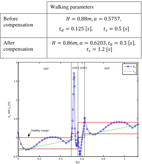
; here and represent local time of the SSP and the DSP respectively. In effect, these parameters have been selected according to previous work which dealt with suboptimal trajectory planning of the same robot model. The proposed hip height of the biped can violate the singularity condition. Therefore, unreasonable solution can be obtained due to appearance of imaginary numbers. Our suggested algorithm tunes the mentioned parameters to give stable trajectory for the COG of biped model. Table 1 shows the walking parameters before and after compensation while Figures 5 and 6 show COG and ZMP trajectories before and after tuning respectively. The results show that after compensation, the hip height will be lower and the biped motion will be slower.

 WP1 vs. WP2.

From Figure 7, it could be noted that the ZMP is out of its stability margin at the beginning of the DSP due to rotation of the rear foot instantaneously at the DSP. This instability can be avoided in WP1 which can guarantee smooth transition or ZMP trajectory and foot rotation. In effect, keeping stance foot fixed at beginning of DSP is necessary to get stable motion.

Table 1. Tuning of walking parameters

Walking parameters

Before compensation

After compensation

Fig. 5: ZMP and COG trajectories before compensation (WP1)

0 0.2 0.4 0.6 0.8 1

-0.5 0 0.5 1 1.5 2

t[s]

px

a

n

d

cx

[

m

]

p_x cx

Stability margin

DSP1 DSP2

Fig. 6: ZMP and COG trajectories after compensation (WP1)

Fig. 7: ZMP and COG trajectories after compensation (WP2)

8.

CONCLUSIONS

In this paper, a simple algorithm has been performed for generating stable biped locomotion. Keeping the stance foot fixed (non-rotated) at beginning of the DSP is important to ensure balanced motion. The disadvantage of our algorithm is that it cannot be applied online because it needs some number

of iterations to get the suitable parameters. An improved version of the algorithm is needed to be applied online in future work.

9.

R

[1] Vukobratovic, M.; Borovac, B. 2004. Zero-moment point-thirty five years of its life. International Journal of Humanoid Robotics, Vol. 1, No. 1, pp. 157-173.

[2] Vanderborght, B.; Van Ham, R.; Verrelst, B.; Van Damme, M.; Lefeber, D. 2008. Overview of the Lucy project: dynamic stabilization of a biped powered by penumatic artifcial mauscles. Advanced Robotics , Vol. 22, No.10, pp. 411-426.

[3] Chevallereau, C.; Bessonnet, G.; Abba, G.; Aoustin, Y. 2009. Bipedal robots: modeling, design and building walking robots. John Wiley and Sons Inc.,.

[4] Vukobratovic, M.; Stepanenko, J. 1972. On the stability of anthropomorphic systems. Mathematical Biosciences, Vol.15, No.1-2, pp.1-73.

[5] Al-Shuka, Hayder F. N.; Corves, B. 2013. On the walking pattern generation of biped robot. Journal of Automation and Control (JOACE), Vol. 1, No. 2, pp.149-155.

[6] Al-Shuka, Hayder F. N.; Corves, B.; Zhu, W.-H. 2013. On the dynamic optimization of biped robot. Lecture Notes on software Engineering, Vol. 1, No. 3, pp. 237-243.

[7] Al-Shuka, Hayder F. N.; Corves, B.; Vanderborght, B.; Zhu, W.-H. 2013. Finite difference-based suboptimal trajectory planning of biped robot with continuous dynamic response. International Journal of Modeling and Optimization, Vol. 3, No. 4, pp. 337-343.

[8] Al-Shuka, Hayder F. N.; Allmendinger, F.; Corves, B.; Zhu, W.-H. 2013. Modeling, stability and walking pattern genartors of biped robots: a review. Robotica, FirstView Article, pp. 1-28.

[9] Kudoh, S.; Komura, T. 2003. C2 continuous gait-pattern generation for biped robots. IEEE/RSJ Intelligent Robots and Systems, vol. 2, pp. 1135-1140. Las Vegas, Nevada.

[10]Shibuya, M.; Suzuki, T.; Ohnishi, K. 2006. Trajectory planning of biped robot using linear pendulum mode for double support phase. Proc. IECON 2006-32nd Annual Conf. IEEE Industrial Electronics, pp. 4049-4099, Paris.

0 0.5 1 1.5 2 2.5

-0.5 -0.4 -0.3 -0.2 -0.1 0 0.1 0.2 0.3 0.4 0.5

t[s]

px

a

n

d

cx

[

m

]

px

c_x

SSP DSP1 DSP2 SSP

Stability margin

0 0.5 1 1.5 2 2.5 3 3.5

-0.5 -0.4 -0.3 -0.2 -0.1 0 0.1 0.2 0.3 0.4 0.5

t[s]

px

a

n

d

cx

[

m

]

px

c_x Stability margin