Markov Chain Monte Carlo to Study the Estimation of
the Coefficient of Variation
M. A. W. Mahmoud
Mathematics Department, Faculty of Science, Al-Azhar University,Nasr City (11884), Cairo, Egypt.
A. A. Soliman
Mathematics Department,Faculty of Science,
Islamic University, Madinah, Saudi Arabia.
A. H. Abd Ellah
Mathematics Department, Faculty of Science, Sohag University,
Sohag 82524, Egypt
R. M. El-Sagheer
Mathematics Department, Faculty of Science, Al-Azhar University,Nasr City (11884), Cairo, Egypt.
ABSTRACT
The coefficient of variation (CV) of a population is defined as the ratio of the population standard deviation to the population mean. It is regarded as a measure of stability or uncertainty, and can indicate the relative dispersion of data in the population to the population mean. In this article, based on the upper record values, we study the behavior of theCV of a random variable that follows a Lomax distribution. Specifically, we compute the maximum likelihood es-timations (MLEs) and the confidence intervals ofCV based on the observed Fisher information matrix using asymptotic distribu-tion of the maximum likelihood estimator and also by using the bootstrapping technique. In addition, we propose to apply Markov Chain Monte Carlo (MCMC) techniques to tackle this problem, which allows us to construct the credible intervals. A numerical ex-ample based on a real data is presented to illustrate the implemen-tation of the proposed procedure. Finally, Monte Carlo simulations are performed to observe the behavior of the proposed methods.
General Terms:
Computer Science Algorithms
Keywords:
Lomax distribution, Coefficient of variation, Markov chain Monte Carlo, Upper record value, Bootstrap.
1. INTRODUCTION
The coefficient of variationcan be used to compare distributions ob-tained with different units, such as, for example, the variability of the weights of newborns (measured in grams) with the size of adults (measured in centimeters). This approach has been used by several authors to obtain theCV estimates see Pang et al. [26] and Pang et al. [27]. TheCV has long been widely used as a descriptive and inferential quantity in several fields such as chemistry, engineer-ing, finance, medical sciences, physics, and telecommunications. In chemical experiments, it is often used as a yardstick of precision
of measurements; two measurement methods may be compared on the basis of their respectiveCV. In finance, theCV can be used as a measure of relative risks (Miller and Karson [24]): In clinical and diagnostic areas, theCV is also often used as a yardstick of the pre-cision of measurements (Reh and Scheffler [29]). In physiological science, theCV can be applied to assess the homogeneity of bone samples (Hamer et al.[17]). It has been used as a tool in uncertainty analysis of fault trees (Ahn [3]) and in assessing the strength of ce-ramics Gong and Li [13]. Many statistical procedures concerning CV are based on the normal distribution. However, several phe-nomena do not agree with the normality assumption due to asym-metry or to the presence of heavy-andlight tails in the distribution of the data. Thus, the statistical inference under normal populations cannot be adequate in the mentioned cases.
The inverse of the coefficient of variation (1/CV), called Sharpe’s ratio or index, is very popular in finance as a measure of portfo-lio performance see Knight and Satchell [19]. The wide use of this index stems from the fact that it is an individual measure of perfor-mance and not an equilibrium one. Since this is a ratio, Sharpe’s index measures the slope of the indifference curve in the mean– standard deviation space so that a higher value of this index im-plies a higher mean–variance expected utility. For applications of Sharpe’s ratio in the analysis of portfolio selection models and in a market risk, see Rachev et al. [28] and Marrison [22]. For a recent illustration of its use in insurance see, Dacorogna and R¨uttener [9]. Bayesian statistical methods provide a complete paradigm for both statistical inference and decision making under uncertainty. This methodology allows to combine information derived from obser-vations with information elicited from experts. The range of its potential applicability is very wide. For example, it is particularly useful for highly reliable components and systems where failures in test and field operations are very rare, requiring the use of all other information. A summary of the Bayesian activity is presented by Berger [6].
business failure data. For its applications as lifetime distribution and extensions, we refer to Marshall and Olkin [21]. Bryson [7] has argued that Lomax distributions provide a very good alternative to common lifetime distributions like exponential, Weibull, or gamma distributions when the experimenter presumes that the population distribution may be heavy-tailed. Details on Pareto distributions as well as areas of application can be found in Arnold [4].
Lomax distribution has been shown to be useful for modeling and analyzing the life time data in medical and biological sciences, en-gineering, etc. So, it has been received the greatest attention from theoretical and applied statisticians primarily due to its use in reli-ability and lifetesting studies. Many statistical methodes have been developed for this distribution, for a review of Lomax distribu-tion see Habibullh and Ahsanullah [15], Upadhyay and Peshwani [32] and Abd Ellah [1,2]. Agreat deal of research has been done on estimating the parameters of a Lomax using both classical and Bayesian techniques.
Therefore, the purpose of this paper is to develops the Bayes es-timates and Markov Chain Monte Carlo (MCMC) techniques to compute the credible intervals and bootstrap confidence intervals of the coefficient of variationCV based on upper record values from the Lomax distribution.
Let XU(1), XU(2), XU(3), ..., XU(n) be the first upper record valuse of sizenarising from a sequence{Xi}of i.i.d Lomax
vari-ables with the probability density function pdf f(x) =αβα(x+β)−(α+1),
x≥0, α, β >0. (1) and cumulative distribution function cdf
F(x) =1−βα(x+β)−α,
x≥0, α, β >0, (2) whereβis the scale parameter andαis the shape parameter. The Lomax distribution has the following properties
(1) The expected value ofX
E(X) =
Z ∞ 0
xf(x)dx
=αβα
Z ∞ 0
x(x+β)−(α+1)dx
= β
(α−1), α >1
(3)
(2) The expected value ofX2
E(X2) =
Z ∞ 0
x2f(x)dx
=αβα
Z ∞ 0
x2(x+β)−(α+1) dx
= 2β
2
(α−1) (α−2), α >2
(4)
The theoretical coefficient of variation under the Lomax distribu-tion is thus given by
CV =
q
E(X2)−(E(X))2 E(X) =
r α
(α−2), α >2.
(5)
The rest of the paper is organized as follows. In Section 2, we dis-cuss the maximum likelihood estimations (MLEs) and the confi-dence intervals ofCV. a Parametric bootstrap confidence intervals are discussed in Section 3. Section 4 describes MCMC for esti-mating the empirical posterior distribution ofCV and its interval estimation. Section 5 contains the analysis of a real life data set to illustrate our proposed method. Simulation studies are reported in order to give an assessment of the performance of the different estimation methods in Section 6. Finally we conclude with some comments in Section 7.
2. MLE OFCV
This section describes the ML method for estimatingCV based on upper record values from the Lomax distribution . Letx=xU(1), xU(2), ..., xU(n) be the first upper record values of sizen from Lomax(α, β).The likelihood function for observed recordxgiven by see Arnold et al. [5]
`(α, β|x) =f(xu(n))
n−1 Y
i=1
f(xu(i))
1−F(xu(i))
. (6)
From Equations (1), (2), and (6), the likelihood function is given by
`(α, β|x) =αnβα(xu(n)+β)−α
n
Y
i=1
(xu(i)+β)−1. (7)
The log-likelihood function may then be written as L(α, β|x) = log`(α, β|x)
=nlogα+αlogβ−
αlog xu(n)+β
−
n
X
i=1
log xu(i)+β
, (8)
by taking derivative in Equation (8) with respect toα,andβ, and equating each result to zero, obtained
∂L(α, β|x)
∂α = n
α+ logβ−log xu(n)+β
= 0 (9) and
∂L(α, β|x)
∂β = α β−
α xu(n)+β
−
n
X
i=1
1
xu(i)+β
= 0. (10) From (9), the ML estimate ofαdenoted byαbis
b
α= n
log xu(n)+β
−logβ (11) By substituting Equation (11) in Equation (10), we get
n
b
βhlogxu(n)+βb
−logβb i−
n
xu(n)+βb h
logxu(n)+βb
−logβb i−
n
X
i=1
1
xu(i)+βb = 0.
(12)
likeli-hood Equation (12) using, for example, the Newton–Raphson iter-ation scheme, and hence the corresponding ML estimateαbof the parameterαis computed from Equation (11) as
b
α= n
log
xu(n)+βb
−logβb
, (13)
then, using the invariance property of the ML estimators, the ML estimate ofCV, denoted byCVˆ , is given by
ˆ
CV =
s
ˆ
α
( ˆα−2),α >ˆ 2. (14)
2.1 Asymptotic likelihood method
To find an asymptotic variance of the ML estimateCVˆ , we shall first write the observed Fisher information matrix V = (vij),
where the partial derivativesvij’s are given by
v11=∂L
2(α, β|x) ∂α2
=−n
α2
(15)
v22=∂L
2(α, β|x) ∂β2
=−α
β2 + α
xu(n)+β 2
+
n
X
i=1
1
xu(i)+β 2
(16)
v12=v21
= ∂L
2(α, β|x) ∂α∂β
= 1
β−
1
xu(n)+β .
(17)
An approximate estimate of the variance-covariance matrix of
ˆ
αandβˆisV−1ij|α,ˆβˆ. In order to find an approximate estimate of the variance ofCVˆ using the Delta method, see Greene [14], let
G0=
∂CV
∂α , ∂CV
∂β
, (18)
where ∂CV ∂α and
∂CV
∂β are the first derivatives of theCV with respect to the parametersαand β. The approximate asymptotic variance ofCVˆ is given by
ˆ
V ar( ˆCV)'hG0I−1Gi|α,ˆβˆ.
The asymptotic distribution of the MLECVˆ ofCV satisfies:
( ˆCV −CV)/ q
ˆ
V ar( ˆCV)∼N(0,1).
This yields that the asymptotic100(1−α)%confidence interval forCV is given by
ˆ
CV ±Z1−γ/2 q
ˆ
V ar( ˆCV). (19)
3. PARAMETRIC BOOTSTRAP CONFIDENCE INTERVALS OFCV
This section discuss two confidence intervals based on the para-metric bootstrap methods: (i) percentile bootstrap method (Boot-p) based on the idea of Efron [10], (ii) bootstrap-t method (Boot-t) based on the idea of Hall [16]. We illustrate briefly how to estimate confidence intervals ofCV using both methods.
1. From the original sample {xU(1), xU(2), ..., xU(n)}, compute MLEs( ˆα,βˆ)of(α, β)andCVˆ ofCV using Equation (14). 2. Using αˆ and βˆ generate a bootstrap sample
{x∗
U(1), x ∗
U(2), ..., x ∗
U(n)}. Use this sample to compute the MLE( ˆα∗,βˆ∗)
of (α, β)andCVˆ ∗ofCV .
3. Repeat step 2,B boot times, to get parametric bootstrap esti-matesCVˆ ∗1, . . . ,CVˆ
∗
BofCV.
In the following, we propose to use two types of parametric boot-strap confidence intervals for theCV.
3.1 Boot-p
Suppose that G(z) = P( ˆCV∗z)be the cumulative distribution function ofCVˆ ∗. DefineCVˆ ∗Boot−p = G
−1
(z)for givenz. The approximate bootstrap100(1−γ)%confidence interval ofCV is given by
ˆ
CV∗Boot−p(
γ
2), ˆ
CV∗Boot−p(1−
γ
2)
. (20)
3.2 Boot-t
Compute the following statisticT∗ =
√
B( ˆCV∗−CVˆ )
q
V ar( ˆCV∗)
.For the
T∗values, determine the upper and lower bounds of the100(1− γ)%confidence interval ofCV as follows: letH(z) =P(T∗≤z)
be the cumulative distribution function ofT∗. For a givenz, define
ˆ
CV∗Boot−t(z) = ˆCV
∗
+B−1/2 q
V ar( ˆCV∗)H−1(z). The approximate100(1−γ)%confidence interval ofCV is given by
ˆ
CV∗Boot−t(
γ
2), ˆ
CV∗Boot−t(1−
γ
2)
. (21)
4. BAYES ESTIMATOR OFCV USING MCMC
By considering model (1), assume the following gamma prior den-sities forαandβas
h1(α|a, b) =
ba
Γ(a)α
a−1exp (−bα) if α >0
0 if α≤0.
(22)
and
h2(β|c, d) =
dc
Γ(c)β
c−1exp (−dβ)
if β >0 0 if β≤0.
(23)
Multiplyingh1(α|a, b)byh2(β|c, d)we obtain the joint prior den-sity ofαandβ; given by
h(α, β) = b
adc
Γ(a)Γ(c)α
a−1 βc−1
exp (−bα−dβ) (24)
Based on the likelihood function of the observed sample is same as (8) and the joint prior in (24), the joint posterior density ofαandβ given the data is
h∗(α, β|x) =R∞ L(data|α, β)×h(α, β) 0
R∞
0 L(data|α, β)×h(α, β)dαdβ
, (25)
therefore, the Bayes estimate of any function of α and β say g(α, β), under squared error loss function is
˜
g(α, β) = Eα,β|data(g(α, β))
=
R∞ 0
R∞
0 g(α, β)L(data|α, β)h(α, β)dαdβ R∞
0 R∞
0 L(data|α, β)h(α, β)dαdβ
.(26)
Generally, the ratio of two integrals given by (26) can not be ob-tained in a closed form. In this case, we use the MCMC method to generate samples from the posterior distributions and then compute the Bayes estimator ofg(α, β)under the squared errors loss (SEL) function. Therefore, we propose the approaches of MCMC tech-nique to approximate (26). See, for example, Robert and Casella [31] and Recently, Rezaei et al. [30].
4.1 MCMC technique
In this subsection we consider the MCMC method to generate sam-ples from the posterior distributions and then compute the Bayes es-timates ofCV of the Lomax distribution under the squared errors loss (SEL) function. A wide variety of MCMC schemes are avail-able, and it can be difficult to choose among them. An important sub-class of MCMC methods are Gibbs sampling and more gen-eral Metropolis-within-Gibbs samplers. The advantage of using the MCMC method over the MLE method is that we can always obtain a reasonable interval estimate of the parameters by constructing the probability intervals based on the empirical posterior distribution. This is often unavailable in maximum likelihood estimation. In-deed, the MCMC samples may be used to completely summarize the posterior uncertainty about the parameters and, through a ker-nel estimate of the posterior distribution. This is also true of any function of the parameters,CV in particular. Suppose we wish to give point and interval estimates forCV .
The expression for the joint posterior can be obtained up to propor-tionality by multiplying the likelihood with the joint prior and this
can be written as
h∗(α, β)∝αn+a−1βα+c−1×
exp[−(bα+dβ+αlog(xu(n)+β)]×
n
Y
i=1
xu(i)+β −1
,
(27)
from (27) it is clear that the posterior density function ofαgivenβ is proportional to
h∗1(α|β)∝αn+a −1×
exp−α
b+ log(xu(n)+β)−logβ
. (28) Therefore, the posterior density function ofαgivenβ, is gamma with parameters (n+a) and b+ log(xu(n)+β)−logβ
. The posterior density function ofβgivenαcan be written as h∗2(β|α)∝β
α+c−1×
exp
"
−dβ−αlog(xu(n)+β)−
n
X
i=1
log(xu(i)+β) #
.
(29) The posterior distribution ofβ givenαEquation (29) cannot be reduced analytically to well known distributions and therefore it is not possible to sample directly by standard methods. We, em-ploy the Metropolis-within-Gibbs method instead to sample. The choice of the hyperparameters (a, b, c, d) are which make (29) close to the proposal distribution and obviously more convergence of the MCMC iteration. We propose the following MCMC algorithm to draw samples from the posterior density functions; and in turn compute the Bayes estimates and also, construct the corresponding credible intervals ofCV.
Algorithm 1.
1. β0=β, Mb =nburn.
2. Generateα1from gamma distributionh∗ 1(α|β).
3. Generateβ1fromh∗2(β|α)using (M-H) algorithm see Metropo-lis et al. [23].
4. ComputeCV1from (14).
5. Repeat steps 2-4N times we obtainCV1,CV2,. . ., CVN.
6. Obtain the Bayes estimate ofCV with respect to the SEL func-tion as
b
E(CV|data) = 1
N−M
N
i=M+1
CVi. (30)
7. To compute the credible intervals of CV, order CVM+1,
CVM+2, ..., CVNas
CV(1), CV(2), ..., CV(N−M) Then the100(1−γ)% symmetric credible intervals
CV((N−M)γ/2), CV((N−M)(1−γ/2))
. (31)
5. ILLUSTRATIVE EXAMPLE
0.96 4.15 0.19 0.78 8.01 31.75 7.35 6.50 8.27 33.91 32.52 3.16 4.85 2.78 4.67 1.31 12.06 36.71 72.89
[image:5.595.323.549.66.239.2]Therefore, we observe the upper record values from the observed data as follows: 0.96, 4.15, 8.01, 31.75, 33.91, 36.71, 72.89. Amodel suggested by engineering considerations is that, for a fixed voltage level, time to breakdown has a Lomax distribution. Based on these seven upper record values, we run the chain for 10 000 times and discard the first 1000 values as ‘burn-in’. When the non-informative prior distribution is used, the joint posterior distribu-tion of the parameters is propordistribu-tional to the likelihooh funcdistribu-tion. The Bayes point estimates and 95% credible intervals forCV are computed. also performed a simple bootstrap procedure to gener-ate the sampling distribution ofCV based on the observed seven upper record values. The point estimates ofCV using the max-imum likelihood method and bootstrap methods as well as 95% bootstrap confidence interval are presented in Table 1. If we adopt the Bayesian approach, we have the results in Table 2. The descrip-tive statistics as well as the 95% credible interval forCV based on the MCMC generated sample are also given in Table 2. As we can see from the histograms of the posterior distributions ofCV in Figure 1.
Table 1. MLE and Bootstrap results ofCV Method CVˆ 95%C.I. Length
MLE 1.7071 [-0.7929, 4.2071] 5.0000 Boot-p 1.9469 [1.2078, 5.1171] 3.9093 Boot-t 1.8439 [0.0896, 3.9770] 3.8874
Table 2. MCMC descriptive statistics ofCV
Mean Median Mode SD
1.9667 1.7969 1.7573 1.0379 Skewness 95%C. I. Length
4.5488 [1.1282, 5.4117] 4.2835 where95%C. I. means that95%Credible Interval.
6. MONTE CARLO SIMULATIONS
In this section, we report some numerical experiments performed to evaluate the behavior of the MCMC methods for different upper record samples froma Lomax distribution, different parameter val-ues, and different priors. Then we use MCMC method to estimate theCV based on10 000samples and discard the first1000values as ‘burn-in’. Thus we can construct the95%confidence intervals. The simulation runs then repeatN = 1000 times. We compute the average Bayes estimates, mean squared errors (MSEs), cover-age percentcover-ages (C.P), and the avercover-age lengths (A.L) based onN replications.
In our present study, we set the different sample sizesn, we also, used two sets of parameter values α = 3, β = 3.1 and α
= 4.2, β = 3.1.We used different hyperparameters(a, b, c, d), mainly to explore their effects on the estimates ofCV. First, we used the noninformative gamma priors for both shape parameters,
(a = b = c = d = 0). Note that as the hyperparameters go to0, the prior density becomes inversely proportional to its argu-ment and also becomes improper. This density is commonly used
Fig. 1. Histogram ofCV
[image:5.595.71.268.295.453.2]as an improper prior for parameters in the range of 0to infin-ity, and this prior is not specifically related to the gamma density. Other than noninformative prior, we also used an informative prior (a= 5, b=c =d = 0.5)for the two sets of parameter values. The simulation results are presented in Tables 3 and 4.
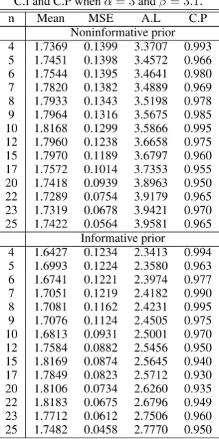
Table 3. MCMC estimates of theCV with MSE, average length of95%
C.I and C.P whenα= 3andβ= 3.1.
n Mean MSE A.L C.P
Noninformative prior 4 1.7369 0.1399 3.3707 0.993 5 1.7451 0.1398 3.4572 0.966 6 1.7544 0.1395 3.4641 0.980 7 1.7820 0.1382 3.4889 0.969 8 1.7933 0.1343 3.5198 0.978 9 1.7964 0.1316 3.5675 0.985 10 1.8168 0.1299 3.5866 0.995 12 1.7960 0.1238 3.6658 0.975 15 1.7970 0.1189 3.6797 0.960 17 1.7572 0.1014 3.7353 0.955 20 1.7418 0.0939 3.8963 0.950 22 1.7289 0.0754 3.9179 0.965 23 1.7319 0.0678 3.9421 0.970 25 1.7422 0.0564 3.9581 0.965
Informative prior
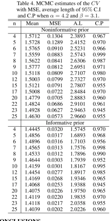
[image:5.595.357.517.376.696.2]Table 4. MCMC estimates of theCV with MSE, average length of95%C.I
and C.P whenα= 4.2andβ= 3.1.
n Mean MSE A.L C.P
Noninformative prior 4 1.5712 0.1304 2.3893 0.967 5 1.5728 0.1289 2.4152 0.970 6 1.5765 0.0910 2.5231 0.966 7 1.5559 0.0883 2.5743 0.999 8 1.5622 0.0841 2.6306 0.987 9 1.5777 0.0812 2.6951 0.971 10 1.5118 0.0809 2.7107 0.980 12 1.5003 0.0799 2.7327 0.970 15 1.5121 0.0791 2.7807 0.955 17 1.5008 0.0722 2.8484 0.970 20 1.4779 0.0705 2.8883 0.960 22 1.4824 0.0686 2.9101 0.961 23 1.4928 0.0627 2.9463 0.945 25 1.4630 0.0573 2.9660 0.955
Informative prior
4 1.4445 0.0320 1.5745 0.970 5 1.4856 0.0317 1.6893 0.968 6 1.4896 0.0316 1.7103 0.956 7 1.4565 0.0313 1.7576 0.998 8 1.4533 0.0312 1.7896 0.990 9 1.4644 0.0303 1.7939 0.952 10 1.4159 0.0301 1.8167 0.995 12 1.4454 0.0277 1.8917 0.985 15 1.4169 0.0268 1.9346 0.965 17 1.4068 0.0253 1.9388 0.945 20 1.4075 0.0226 1.9750 0.965 22 1.4119 0.0220 1.9835 0.970 23 1.4118 0.0217 2.0358 0.955 25 1.4039 0.0202 2.0226 0.960 7. CONCLUSIONS
This article study the estimation of theCV of a random variable that follows a Lomax distribution, when the available data are up-per record values. Maximum likelihood, parametric bootstrap and MCMC Bayes methods are proposed, to obtain point estimates, as well as confidence intervals of theCV. We introduced illustrated example using the observed sample of real data. We found that the Bayes estimates cannot be obtained in explicit form. We used the MCMC technique to compute the approximate Bayes estimates and the corresponding credible intervals.
From results in Tables 1 and 2, we observed that most of the meth-ods work well in general. The MCMC method provides an alter-native method for parameter estimation of the Lomax distribution. Indeed, the MCMC sample may be used to completely summaries posterior uncertainty about the parameters, through a kernel esti-mate of the posterior distribution. Bayes estiesti-mates of the unknown parameters and then theCV can be obtained using Gibbs sampling and the Metropolis-Hastings procedures.
A simulation study was conducted to examine the performance of the MCMC Bayes estimators for different parameters values, different sample size (n) and different priors. We observe that, comparing the two Bayes estimators based on noninformative and informative priors clearly shows that the Bayes estimators based on informative prior perform better than the Bayes estimators based on noninformative prior , in terms of both MSEs and the length of the credible intervals.
8. REFERENCES
[1] A. H. Abd Ellah,Bayesian one sample prediction bounds for the Lomax distribution, Indian J. Pure Appl. Math.42(2011), no. 5, 335–356.
[2] A. H. Abd Ellah,Comparison of estimates using record stat-stics from Lomax model : Bayesian and non Bayesian ap-proaches, J. Stat. Res. Train. Center3(2006), 139-158. [3] K. Ahn,Use of coefficient of variation for uncertainty
anal-ysis in fault tree analanal-ysis, Reliab. Engin. System Safety47 (1995), no 3, 229–230.
[4] B. C. Arnold, Pareto Distributions. In: Statistical Distribu-tions in Scientific Work, International Co-operative Publishing House, Burtonsville, MD, 1983.
[5] B. C. Arnold, N. Balakrishnan and H. N. Nagaraja,Records, Wiley, New York, 1998.
[6] J. O. Berger,Statistical Decision Theory and Bayesian Anal-ysis. New York, Springer Verlag, 1985.
[7] M. C. Bryson, Heavy-tailed distributions: properties and tests, Technometrics16(1974), no. 1, 61–68.
[8] M. Chahkandi and M. Ganjali,On some lifetime distributions with decreasing failure rate, Comput. Statist. Data Anal.53 (2009), no. 12, 4433–4440.
[9] M. M. Dacorogna and E. R¨uttener, Why time-diversified equalisation reserves are something worth having, Con-verium Research Report, Switzerland, 2006.
[10] B. Efron, The bootstrap and other resampling plans, In: CBMS-NSF Regional Conference Seriesin Applied Mathe-matics, SIAM, Philadelphia, PA, 1982.
[11] S. Geman and D. Geman,Stochastic relaxation, Gibbs distri-butions, and the Bayesian restoration of images, IEEE Trans. Pattern Anal. Mach. Intell.6(1984), 721–741.
[12] W. R. Gilks, S. Richardson and D. J. Spiegelhalter,Markov chain Monte Carlo in Practices, Chapman and Hall, London, 1996.
[13] J. Gong and Y. Li,Relationship between the estimated Weibull modulus and the coefficient of variation of the measured strength for ceramics,J. Ame. Ceramics Society,82(1999), no. 2, 449–452.
[14] W. H. Greene,Econometric Analysis, 5th Ed. New York Uni-versity, 2002.
[15] M. Habibullah, and M. Ahsanullah,Estimation of parameters of a Pareto distribution by generalized order statstics, Comm. Statist. Theory Methods29(2000), 1597-1609.
[16] P. Hall,Theoretical comparison of bootstrap confidence inter-vals, Ann. Stat.16(1988), 927-953.
[17] A. J. Hamer, J. R. Strachan, M. M. Black, C. Ibbotson and R. A. Elson,A new method of comparative bone strength mea-surement, J.Med. Engin.Tech.19(1995), no. 1, 1–5. [18] W. K. Hastings, Monte Carlo sampling methods using
Markov chains and their applications, Biometrika57(1970), 97–109.
[19] J. Knight and S. Satchell,Are-examination of Sharpe’s ratio for log-normalprices, Appl. Math. Finance,12(2005), no. 1, 87–100.
[20] K. S. Lomax,Business failure: Another example of the anal-ysis of the failure data, JASA49(1954),847-852.
[22] C. Marrison, The Fundamentals of Risk Measurement, McGraw-Hill, New York, 2002.
[23] N. Metropolis, A. W. Rosenbluth, M. N. Rosenbluth, A. H. Teller and E. Teller,Equations of state calculations by fast computing machines, J. Chem. Phy.21(1953), 1087–1091. [24] E. G. Miller and M. J. Karson,Testing Equality of Two
Coef-ficients of Variation, Amer. statist. Assoc. Posceed. Business and economics1(1977), 278-283.
[25] W. B. Nelson,Applied Life Data Analysis, Wiley, New York, 1982.
[26] W. K. Pang, W. T. Y. Bosco, M. D. Troutt and H. H. Shui,A simulation-based approach to the study of coefficient of vari-ation of dividend yields, European J. Oper. Res.189(2008), 559–569.
[27] W. K. Pang, P. K. Leung, W. K. Huang and W. Liu, On interval estimation of the coefficient of variation for the three-parameter Weibull, lognormal and gamma distribution: A simulation based approach, European J. Oper. Res. 164 (2005), 367–377.
[28] S. T. Rachev, I. Huber and S. Ortobelli, Portfolio choice with heavy tailed distributions. Tech. Rep., University of Karl-sruhe, Germany, 2004. .
[29] W. Reh, and B. Scheffler,Significance tests and confidence intervals for coefficient of variation,Comput. Stat. Data Anal. 22(1996), no. 4, 449–453.
[30] S. Rezaei, R. Tahmasbi and M. Mahmoodi,Estimation of P[Y¡X] for generalized Pareto distribution, J. Statist. Plann. Inference,140(2010), 480-494.
[31] C. P. Robert and G. Casella,Monte Carlo Statistical Methods, Second edition, Springer, New York, 2004.