BIROn - Birkbeck Institutional Research Online
Garnier, P. and Holmberg, M.K.G. and Wahlund, J.-E. and Lewis, G.R. and
Grimald, S.R. and Thomsen, M.F. and Gurnett, D.A. and Coates, Andrew J.
and Crary, F.J. and Dandouras, I. (2013) The influence of the secondary
electrons induced by energetic electrons impacting the Cassini Langmuir
probe at Saturn. Journal of Geophysical Research: Space Physics 118 (11),
pp. 7054-7073. ISSN 2169-9380.
Downloaded from:
Usage Guidelines:
Please refer to usage guidelines at or alternatively
JOURNAL OF GEOPHYSICAL RESEARCH: SPACE PHYSICS, VOL. 118, 7054–7073, doi:10.1002/2013JA019114, 2013
The influence of the secondary electrons induced by energetic
electrons impacting the Cassini Langmuir probe at Saturn
P. Garnier,1,2M. K. G. Holmberg,3J.-E. Wahlund,3 G. R. Lewis,4,5S. Rochel Grimald,1,2,6 M. F. Thomsen,7 D. A. Gurnett,8 A. J. Coates,4,5F. J. Crary,9and I. Dandouras1,2
Received 11 June 2013; revised 12 September 2013; accepted 22 October 2013; published 15 November 2013.
[1] The Cassini Langmuir Probe (LP) onboard the Radio and Plasma Wave Science experiment has provided much information about the Saturnian cold plasma environment since the Saturn Orbit Insertion in 2004. A recent analysis revealed that the LP is also sensitive to the energetic electrons (250–450 eV) for negative potentials. These electrons impact the surface of the probe and generate a current of secondary electrons, inducing an energetic contribution to the DC level of the current-voltage (I-V) curve measured by the LP. In this paper, we further investigated this influence of the energetic electrons and (1) showed how the secondary electrons impact not only the DC level but also the slope of the (I-V) curve with unexpected positive values of the slope, (2) explained how the slope of the (I-V) curve can be used to identify where the influence of the energetic electrons is strong, (3) showed that this influence may be interpreted in terms of the critical and anticritical temperatures concept detailed by Lai and Tautz (2008), thus providing the first observational evidence for the existence of the anticritical temperature, (4) derived estimations of the maximum secondary yield value for the LP surface without using laboratory measurements, and (5) showed how to model the energetic contributions to the DC level and slope of the (I-V) curve via several methods (empirically and theoretically). This work will allow, for the whole Cassini mission, to clean the measurements influenced by such electrons. Furthermore, the understanding of this influence may be used for other missions using Langmuir probes, such as the future missions Jupiter Icy Moons Explorer at Jupiter, BepiColombo at Mercury, Rosetta at the comet Churyumov-Gerasimenko, and even the probes onboard spacecrafts in the Earth magnetosphere.
Citation: Garnier, P., M. K. G. Holmberg, J.-E. Wahlund, G. R. Lewis, S. R. Grimald, M. F. Thomsen, D. A. Gurnett, A. J. Coates, F. J. Crary, and I. Dandouras (2013), The influence of the secondary electrons induced by energetic electrons impacting the Cassini Langmuir probe at Saturn,J. Geophys. Res. Space Physics,118, 7054–7073, doi:10.1002/2013JA019114.
1. Introduction
[2] The Langmuir probe—referred to as LP in the paper— onboard the Cassini spacecraft is part of the Radio and Plasma Wave Science (RPWS) instrument [Gurnett et al., 2004]. It has brought much information about the cold and dense plasma in the Saturnian system since 2004, in
par-1Université de Toulouse; UPS-OMP; IRAP; Toulouse, France. 2CNRS; IRAP, Toulouse, France.
3Swedish Institute of Space Physics, Uppsala, Sweden.
4Mullard Space Science Laboratory, University College London,
Dorking, UK.
5The Centre for Planetary Sciences at UCL/Birkbeck, London, UK. 6Onera-The French Aerospace Lab, Toulouse, France.
7Planetary Science Institute, Tucson, Arizona, USA.
8Department of Physics and Astronomy, University of Iowa, Iowa City,
Iowa, USA.
9Laboratory for Atmospheric and Space Physics, University of
Colorado, Boulder, Colorado, USA.
Corresponding author: P. Garnier, IRAP, 9, avenue du Colonel Roche, BP 44346, 31028 Toulouse cedex 4, France. (Philippe.Garnier@irap.omp.eu)
©2013. American Geophysical Union. All Rights Reserved. 2169-9380/13/10.1002/2013JA019114
ticular regarding the Titan ionosphere [e.g.,Wahlund et al., 2005a; Ågren et al., 2007; Garnier et al., 2009; Edberg
et al., 2011]. The LP also allowed to study the Saturnian
plasma disk [Wahlund et al., 2005b;Morooka et al., 2009;
Gustafsson and Wahlund, 2010] or dusty regions such as the
Enceladus plume or the rings environment [Wahlund et al., 2009;Morooka et al., 2011].
[3] The LP is dedicated to the investigation of cold (below electron temperatures of 5eV) and dense (above sev-eral particles per cubic centimeter) plasmas.Garnier et al.
[2012b], however, also revealed a strong sensitivity of the LP measurements to the energetic electrons (the adjective “energetic” will refer to energies around 250–450 eV in this paper). The analysis of the ion side current (current for negative potentials) measured by the probe showed indeed a correlation with these energetic electrons, which impact the surface of the LP and generate a detectable current of secondary electrons. The spatial distribution of the 250– 450 eV electrons in the magnetosphere [DeJong et al., 2011] then lead Garnier et al. [2012b] to observe a broad sec-ondary electron current region in the dipoleLshell range of
[4] The purpose of our study is to understand in more detail why this current exists and how we can model it. This will allow either to infer valuable information about the plasma or to remove this current from the measure-ments (it may be considered as a parasite current for the cold plasma investigations). Garnier et al. [2012b, hereinafter G12] indeed identified the source particles of the measured current through a correlation analysis but did not reproduce the current itself. Moreover, the authors focused only on the contribution by the energetic particles on the DC level of the current-voltage curve of the LP (the so calledIenercurrent).
We will, however, show here that the energetic particles also impact the slope of this curve by adding a contributionbener.
[5] The paper is organized as follows: section 2 will describe the instruments and data sets used in our study; section 3 will focus on the slope of the current-voltage curve measured by the LP and its interpretation; sections 4 and 5 will then describe two different methods (respec-tively, empirical and theoretical) to model the impact of the energetic electrons (bothIenerandbenercontributions); a
com-parative discussion on the various modeling methods will be given in section 6; a summary will end the paper in section 7, followed by an Appendix A with the derivation of the equations used.
2. Description of the Data
[6] This section will first present the time intervals used in our study (section 2.1). It will then describe the data used from the LP experiment (section 2.2; see Gurnett et al.[2004] for a description of the LP) and from the CAPS (Cassini Plasma Spectrometer) experiment (section 2.3; see
Young et al.[2004] for a description of CAPS). The time
intervals used here are identical to those discussed in G12; we thus also refer the reader to sections 2 and 3 of G12 for detailed explanations.
2.1. Description of the Time Intervals Used
[7] The time intervals chosen in this paper correspond to the two types of studies presented here: event analysis and statistical study over several years of data. The data sets were chosen to focus on regions where the influence of the ener-getic electrons is the strongest, but one should keep in mind that this influence may be seen in a large part of the magne-tosphere. We will first present the event data set and then the statistical study one.
[8] The case studies chosen include the inbound part of the SOI (Saturn Orbit Insertion) in 2004 and a high-inclination orbit in 2008. During the inbound part of SOI (30 June 2004 at 16:00–20:00 UT), the Cassini spacecraft was located outside the dust region where our analysis would be too complex (see section 2.2.2.1). It was also located inside the secondary electron current region identified in G12, i.e., in the L shell range of 7–10 and at Z values below–1.2RS (RS = 60, 268km Saturn radius). (X, Y,Z)
is the Saturn-centered equatorial coordinate system, withZ pointing northward along Saturn’s spin axis andXin the Sat-urn equatorial plane positive toward the Sun. The second period occurred during a high-inclination orbit on 17 and 18 May 2008, respectively, at 19:30–20:10 UT and 1:40– 2:10 UT during the inbound and outbound legs of the orbit. The spacecraft was located in the same region (withLshell
ranges of 7.4–9.9 and 7–9.6, respectively) and well off the equator at|Z|values above2.75and2.45RS, respectively.
[9] The large data set used for the statistical study consists of all the time intervals of the LP (more than 250,000 time intervals) from 1 February 2005 to 30 July 2008. Several selections of the large data set (with various added criteria, e.g., on the electron temperature or|Z|values) will be used through the paper to extract the most appropriate data inside this large data set.
[10] The time intervals considered in the paper will always be those of the LP. All CAPS data were linearly interpolated to these time intervals. The influence of the interpolation process (induced by the different time resolu-tions between the LP and CAPS data) will be discussed in section 2.3.1.2.
2.2. Langmuir Probe Data
2.2.1. The Currents Measured by the LP
[11] The LP is a titanium nitride (TiN)-coated conductive titanium sphere. A bias voltage (UB) is actively applied to
the LP with respect to the spacecraft in order to detect the electrons or ions, depending on the sign of the potentialU relative to the plasma (U=UB+Vfloat;Vfloatbeing the floating
potential of the probe, considered uniform around the probe
[Nilsson, 2009]). The bias voltage varies between–32 and
+32V in the magnetosphere. This allows the LP to detect the whole distribution of cold electrons or low velocity ions and to determine their characteristics. This does, however, not prevent the impact by energetic particles (e.g., hundreds of eV electrons) that cannot be repelled.
[12] The derivation of the cold plasma parameters (e.g., electron densityneand temperatureTe) is performed through
the fitting of the current-voltage (I-V) curve [Fahleson et al., 1974] using the Orbital Motion Limited (OML) theory
[Mott-Smith and Langmuir, 1926]. The usage of the OML
theory is here justified since our study investigates the thin Saturnian magnetospheric plasma whose Debye length is much larger than the probe radius: e.g., the Debye length is typically above2.5m (compared with the LP radius of
0.025m) at the equator nearL = 6for a density of30cm–3
and a temperature of 4 eV [Persoon et al., 2009].
[13] The ion side current (I–) measured for a negative
potential (U) is given by
I–=Iions+Iel+I*+Idust+Iph+Isecd +I *
sec (1)
whereIionsandIelare the (thermal and ram) currents,
respec-tively, due to the ambient cold ions and electrons,Idustis the
direct charged dust current to the probe,I*the current due
to the direct impact of energetic electrons and ions,Iph the
photoelectron current due to the photoionization of the probe surface,Id
sec the current of secondary electrons induced by
the impact of dust, andI*
secthe current of secondary electrons
induced by the impact of energetic particles.
[14] Only the ram/thermal ion and photoelectron currents are usually considered for negative probe potentials, since the cold electrons are repelled by the negative potential of the probe, the dust is located in specific regions near the equator, and the contribution by the energetic particles (both I* and I*
sec) is typically neglected. G12 showed, however,
GARNIER ET AL.: ENERGETIC ELECTRONS AND THE CASSINI LP
aims at modeling as precisely as possible the current due to the energetic electrons and then being able to remove it from the observations.
[15] The current for negative potentials I– actually
depends linearly on the bias potential at large negativeUB
values, so thatI–is parametrized by a linear equation during
the data analysis process:
I–=m–bUB (2)
where m and b are, respectively, the DC level (corrected for the spacecraft attitude) and slope of the fitted current-voltage curve on the ion side. These two parameters are the most important observables of the LP and then used to derive the plasma parameters. We will show later in our study that (and how) the energetic particles impact both the DC level m(through the addedIenercurrent identified by G12) and the
slopeb(through a contributionbener; see section 2.2.2).
[16] The m current has a random noise level of 0.1nA (measured in laboratory; Wahlund, private communication). The derivation of the photoelectron current induces both a random noise level of 0.05nA and a possible systematic error below0.1nA [Holmberg et al., 2012; Holmberg, pri-vate communication]. The systematic error may be induced by several issues which are today not taken into account, such as a partial shadowing of the probe surface from a boom or an antenna and partial ring eclipses.
2.2.2. Extracting the Energetic DC Level (Iener) and Slope (bener)
[17] As demonstrated by G12, the energetic 250–450 eV electrons impacting the probe generate secondary electrons and modify the current measured by the LP for nega-tive potentials. This does not impact only the DC levelm (through theIenercurrent identified by these authors) but also
the slopebof the current-voltage curve (through an added contributionbener). Understanding this influence implies first
that we are able to extract both Iener and bener from the
measurements.
2.2.2.1. ExtractingIener
[18] The current Iener induced by the energetic particles
impacting the probe—through the direct impact (I*) and the
secondary electrons produced (I*
sec)—may be extracted as
follows from the LP measurements (see section 3 of G12 for the full development):
Iener=m+bVfloat–Ii0–Iph (3)
withIi0 the “random ion current” defined byIi0 =Iions+bU
and given by the various contributions of eachith ion species [Fahleson et al., 1974]:
Ii0= –
X
i
ALPqini
s
v2
i
16+
kBTi
2mi
(4)
withALP the surface of the probe, kB the Boltzmann
con-stant, andni,Ti,qi,vi, andmithe density, temperature, charge
state (essentially+eat Saturn, withethe electron charge), drift speed (in the frame of the LP), and mass of theith ion species. The ion parameters are not provided for each ion species by the LP: it can provide global (density weighted) values but cannot separate the contribution of each species.
[19] The usage of equation (3) to extract the currentIeneris
based, beyond the analysis of the LP observations, on several assumptions:
[20] 1. The dust-induced currents Idust and Isecd shall be
negligible to derive equation (3); Wang et al. [2006] and
Tsintikidis et al. [1994] showed that the dust is confined
inside a layer of 1000–3000 km thickness around the equa-tor; the influence of the dust currents will thus be removed if we focus on regions off the equator (e.g.,|Z| > 1RS).
[21] 2. The photoelectron current Iph shall be properly
estimated; the values derived byHolmberg et al.[2012] were used in our analysis; moreover, all data occurring in eclipse for the LP (including the eclipses due to the spacecraft) were removed from the data set.
[22] 3. The cold ion thermal or ram currentIi0, which is
strong near the equator where the dominating water group ions are centrifugally confined [Sittler et al., 2008], must also be taken into account in principle; the first method is to choose time periods were the spacecraft is so far above the equator (e.g.,|Z| > 2RS; see section 2.3.2 for more details)
that one can neglect this current compared to the other cur-rents; the second method is to calculate the current based on the knowledge of the various parameters included inIi0 (in
particular the ion parameters described in section 2.3.2). [23] For the chosen case studies, all these stages were performed for extractingIener, with theIi0 contribution
cal-culated from the knowledge of the CAPS ion parameters described in section 2.3.2. However, as this procedure is complex, it cannot be applied to the large data set and a simpler method will be used, whereIeneris approximated by
mion = m–Iph. The contributions bybVfloat andIi0 will
indeed be neglected in equation (3) based on the following arguments. The contribution ofbVfloatis negligible
com-pared withm:bis of the order of10–3–10–2nA/V andV float
is of the order of a few volts, whereasmis of the order of
0.5–1.5nA (see Figure 5). Moreover, the contribution of the thermal ions viaIi0 may be neglected as soon as the data
close to the equator are removed (see section 2.3.2). 2.2.2.2. Extractingbener
[24] The influence of the energetic particles is neglected in the Langmuir probe measurements discussed in the lit-erature, and this is particularly true regarding the slope b of the current-voltage curve. As it will be discussed indeed in section 3, we found unexpected values of theb slope, precisely in the secondary electron current region where the currentIener was identified by G12. We will show (see
sections 3, 4, and 5) that the energetic electrons also impact the slope through a contributionbenerdefined by
b=bions+bener (5)
wherebionsis the classic contribution of the ambient ions to
the slopebof the current-voltage curve, given by [Fahleson et al., 1974;Holmberg et al., 2012]:
bions= –
X
i
ALPqini
s
v2
i
16 +
kBTi
2mi
e miv2i/2 +kBTi
(6)
[25] Extracting the contributionbeneralso implies the same
assumptions as for the extraction ofIener(see section 2.2.2.1).
The originalbvalue will, however, be used for the analysis of the large data set, sincebis close tobenerwhen we focus
on the data where the spacecraft is off the equator (|Z| > 2RS)
2.3. The Cassini CAPS Electron and Ion Data 2.3.1. The Electron Data
[26] Three different types of CAPS ELS (ELectron Spec-trometer) electron data were used in this paper and will be described below, corresponding to three different methods (detailed in sections 4 and 5 and compared in section 6) to reproduce the observedIener and bener contributions: the
full electron distribution over all CAPS ELS channels, the average differential number fluxes (keV cm2sr s)–1over the
253–474 eV electrons only (which were identified by G12 as driving the currentIener), and the electron moments (ne,Te).
[27] The first two data sets are identical to the data used in G12. The three types of data will be used for both the case studies and the large data set (defined in section 2.1), except the full distribution which could not be extracted for the large data set given the size of the files associated. More-over, we used only the CAPS data from anode 5, which is the least affected by the spacecraft structures.
2.3.1.1. The Full CAPS ELS Distribution
[28] The full electron distribution is used for the case studies (SOI and high-inclination orbit). It consists of the differential number fluxes (keV cm2sr s)–1 of all 63 energy
channels from 0.53eV/q (lower value of bin number 63) up to 28.3keV/q (upper value of bin number 1). These data were corrected neither for noise (on the contrary to the other data sets; see below) nor for other artifacts such as the obscuration of parts of the spacecraft bus or the focusing of electrons in the nonuniform spacecraft poten-tial. However, insofar as our study focuses on the secondary electron current region (i.e., outside the radiations belts), the noise which might affect our investigation essentially comes from the spacecraft radioisotope thermoelectric genera-tors. This background noise level was estimated byArridge
et al.[2009] at 20–30 counts/s for anode 5 used in our paper
[seeArridge et al., 2009, Figure A2 in Appendix A].
Dur-ing the case studies, the mean signal-to-noise ratio (ratio between the counts/s measured and the counts/s noise level) decreased from 240 to3.1 with the energy (i.e., from bin number 63 to bin number 1), assuming a noise level value of
30counts/s. In particular, the mean signal-to-noise ratio was 32–33 for 253–474 eV electrons. In addition, the data were averaged over 60 s time periods before the interpolation to the LP time intervals. The results discussed later for the case studies will thus not be affected by the noise sources. 2.3.1.2. The 253–474 eV Electrons
[29] The differential number fluxes discussed above were averaged during the case studies over channels 34 to 37 (energies between 253 and 474 eV) to obtain a mean flux value with a 1 min resolution. We remind that this energy range corresponds to the peak energy of the secondary elec-tron yield function for the surface of the LP. This explains why G12 observed a strong correlation between the detected currentIenerand these energetic electrons.
[30] We also used the same energy range for the large data set from 2005 to 2008. The differential number fluxes were, however, averaged over 10 min time intervals given the size of the file associated: 207,542 time intervals, includ-ing the whole orbits and not only the crossinclud-ings of the secondary electron current region. During this large period, we removed all the time intervals where the signal-to-noise ratio was below 1 (for a noise level of30counts/s), which concerned about3.5% of the total data set.
[31] The CAPS electron data were averaged—over 1 min for the case studies or 10 min time intervals for the large data set—before they were interpolated at the LP time inter-vals. The influence of this procedure was analyzed for the mean 253–474 eV electron fluxes during the case studies. After the interpolation at the LP time intervals, we calculated the relative difference between the initially 1 min averaged fluxes and alternative data sets, such as the 15 or 30 s aver-aged fluxes or the 15 s median fluxes. The resulting relative difference after the interpolation process is of the order of 3.4–6.4% only. As a consequence, the difference between the initial time intervals of the CAPS and LP experiments, as well as the choice of the averaging process before the interpolation, will only very slightly impact our results. 2.3.1.3. The Electron Moments
[32] The third type of CAPS data used in this study is the 3D electron moments (ne,Te) derived byLewis et al.[2008].
We first selected the data between 5 June 2004 and the end of 2008 (more than 4 million of time intervals with a time res-olution of 32 s). The moments were then interpolated to the LP time intervals, both for the case studies and the statistical analysis from 2005 to 2008.
[33] The moments are not to be trusted for negative val-ues of the spacecraft potential, also given by Lewis et al.
[2008]. More precisely, since the lowest energy detected by CAPS is 0.6 eV, a threshold at0.6V or—to avoid checking for the number of counts measured—at1V is appropriate to avoid the data which cannot be trusted (G. Lewis, pri-vate communication). A threshold at1V was used for the large data set but not for the case studies, where two thirds of the time intervals should be removed. The spacecraft potential is indeed between0.5 and1V during two thirds of the case studies time intervals. However, the electron moments are still correct during the time intervals, since the potential is still positive and the number of counts/second is large (always above 270) during both the SOI and high-inclination periods.
2.3.2. The Ion Data
[34] As explained in section 2.2.2, the extraction of the energetic contributionsIener andbener to the respective DC
level and slope of the current-voltage curve needs the esti-mation of the thermal ion parameters (see equations (4) and (6)).
[35] We used, for the analysis of the case studies, the ion data published by Sittler et al. [2006] for the SOI period and those published byThomsen et al.[2010] for the high-inclination orbit (M. Thomsen, private communication). The ion data were then interpolated to the LP time intervals.
The Sittler et al. [2006] results include both water group
ions (mW = 17amu) and protons (mH = 1amu), whereas
Thomsen et al. [2010] also include the contribution ofH+
2
ions (mi/qi = 2). Both works provide the following
param-eters for each ion species:ni,Ti, andvi.vi was determined
from the three components of the velocity vector (radial, azimuthal, and vertical) except for the SOI period where
Sittler et al.[2006] assumed a zero vertical velocity. [36] The thermal ions contribute to the DC level (m) and slope (b) of the current-voltage curve through the respective Ii0 and bions parameters. These contribute, respectively, on
GARNIER ET AL.: ENERGETIC ELECTRONS AND THE CASSINI LP
Figure 1. Example of sweep for the LP (18 December 2007 at 21:13 UT), with the current measured as a function of the bias voltageUBapplied to the probe. (top) The whole sweep and (bottom) the negative
potential part. At negative potentials, the probe attracts essentially ions but shows an unusual positive slopeb.
the slope, in particular during SOI where the spacecraft was located closer to the equator (with|Z|1.2RS) than during
the high-inclination periods (where|Z|2.45RS).
[37] We introduced the influence of the thermal ions in the analysis of the case studies but not for the large data set given the complexity of the ion parameters derivation. This will not impact our results regarding the DC level, and the impact will still be small for the slope by selecting periods where the spacecraft was above2RSoff the equator.
3. Unusual Positive Values for the Slope of the Current-Voltage Curve
[38] In this section, we will show and interpret the obser-vations of unusual positive values of the b slope of the current-voltage curve of the LP, observed mostly in the secondary electron current region.
3.1. The Langmuir Probe Observations
[39] The active application to the LP of a variable bias potential UB between –32 and +32V (called a “sweep”)
leads to the plotting of the current-voltage curve. For nega-tive potentials, this curve may be fitted by a linear function (see equation (2)) whose slopebis given by
b= –I(UB= –5 V) –I(UB= –32 V)
–5 + 32 (7)
[40] Since the currents for incoming ions are defined as negative (respectively, positive for incoming electrons), more negative UB values lead to more negative currents
due to more attracted ions, which in the end gives negative values for b. This is also expected from theory, since we classically haveb=bionswherebionsis negative according to
equation (6). The current-voltage curve thus usually shows a
negative value of the slopeb, as observed in any ionosphere (see examples of such curves byWahlund et al.[2005a] or
Ågren et al.[2007] at Titan).
[41] However, as can be seen in Figure 1, we can find LP sweeps wherebis actually positive. This figure shows the current-voltage curve measured on 18 December 2007 at 21:13 UT. Figure 1 (top, left) corresponds to negative poten-tials U, where the ions are attracted. The slope b is thus clearly positive.
[42] Figure 2 shows the occurrence of such events as a function of theL shell, for the large data set with all LP data from 1 February 2005 to 30 July 2008. The figure also gives the radial profile of the normalized electron differen-tial number fluxes (for the energy range 253–474 eV) for the same period. The observed profiles are very similar to those in G12 (Figure 4) which compared the estimatedIener
and the same electron number fluxes. The presence of pos-itive values ofb is indeed very common (up to 83% of the data) in the secondary electron current region off the equator, where the energetic electrons fluxes are high. Such events may even still be seen in the outer magnetosphere, with a smaller occurrence though. Furthermore, mapping the bparameter as a function of bothLshell and local time (not shown) gives also a similar distribution to the one ofIener
in Figure 1 of G12. Such a mapping indeed reveals values larger on the nightside than on the dayside, which is related to the asymmetries observed for the hundreds eV electrons
byDeJong et al.[2011].
[43] One can thus conclude that the energetic electrons impact not only the DC level of the current-voltage curve at negative potentials (through the contributionIener) but also
the slopebof this curve (through a contributionbenerdefined
Figure 2. Occurrence (in percent) of positive values of the slopebas a function ofLshell, for all LP data from 1 February 2005 to 30 July 2008. The red, black, and magenta lines represent, respectively, the occurrences for all time intervals, those with Cassini near the equator, and those off the equator. Two different limits were used for the definition of “equatorial data” and “off equator data”:|Z| > 1RS
(o symbol) and|Z| > 2RS (* symbol). The cyan line gives the normalized CAPS electron differential
number fluxes (keV cm2sr s)–1for the energy range 253–474 eV. The thick blue and red vertical dashed
lines show theLshell values of Dione and Rhea.
3.2. Interpretation
3.2.1. The Balance Between the Incident and Secondary Electrons
[44] The observation of positive slopes of spacecraft current-voltage curves has already been discussed in the past, in particular in the context of the “triple roots” situa-tions. The charging of a spacecraft indeed obeys the current balance equation with all incoming and outgoing currents. This equation is satisfied for a specific potential (floating potential) that is a root for the equation.Whipple[1965] and
Prokopenko and Laframboise[1980] showed that in some
cases, the presence of secondary electrons may induce rever-sals of the current-voltage curve. It may also lead to several roots, with the spacecraft thus jumping from a floating potential to another.
[45] Our positive slope observations can be explained as follows. On the negative side (negative potentials) of the current-voltage curve, the current due to the collected ions (Iions; defined negative) increases in absolute value at large
negative potentials, since the surface attracts more and more ions. This leads to a classical negative slopebas defined by equations (6) and (7). In the same time, the incident electrons are more and more repelled andIel (defined positive) thus
decreases at large negative potentials. The secondary elec-trons current induced by the impact of the incident elecelec-trons (defined negative) also decreases in absolute value since there are less incident electrons. Consequently, if there are more secondary than incident electrons (i.e., if the secondary electron yield is greater than 1), then the total (incident + sec-ondary) electron current is negative and has a positive slope. In the end, if the ion current is smaller than the total (inci-dent + secondary) electron current, the slopebobserved will be positive.
[46] Figure 3 shows a zoom of the current-voltage curve example previously shown in Figure 1, where we added
the individual current contributions. The ion contribution Iions (not shown) may be neglected since the spacecraft is
far off the equator (Z2.6RS). The total current due to the
energetic electrons—incident + secondary electrons—was modeled with the theoretical moments approach described later in detail (see section 5 and equation (11) in particular). Adding this contribution to the photoelectrons current Iph
allows to reproduce very closely the measurements. 3.2.2. Identification of the Critical/Anticritical Temperatures
[47] The key factor leading to positive slopes is the pres-ence of more secondary than incident electrons. The ratio between secondary and incident electrons as a function of the energy is given for any material by the secondary elec-tron emission yield (SEEY). This yield is known to peak (with a yield above one) at incident electron energies near 200–1000 eV for metal layers [Hastings and Garrett, 1996]. The peak energy for the Cassini LP was determined by G12 close to 350 eV, in agreement with laboratory measu-rements of TiN surfaces by Walters and Ma [2001] or
Lorkiewicz et al.[2007]. The exact form and the maximum
yield value are, however, essentially unknown and will be discussed further in sections 5.1.2.1 and 5.3.
[48] Laframboise et al.[1982] andLai et al.[1983] were
the first to introduce the concept of “threshold tempera-ture” or “critical temperatempera-ture” for the spacecraft charging. The SEEY curve indeed implies the existence of an elec-tron temperature of the ambient plasma below which there will be less incident than secondary (and backscattered) elec-trons. A surface material thus cannot be charged negatively in this plasma environment. Above the critical tempera-ture T* specific for each surface composition, one may
GARNIER ET AL.: ENERGETIC ELECTRONS AND THE CASSINI LP
Figure 3. Negative potential side of the Figure 1 current-voltage curve obtained on 18 December 2007 at 21:13 UT. The total measuredI–current (blue dots) is compared with the modeledI– current (black
line) derived from the addition of the photoelectron current (Iph, green line) and the current due to the
energetic electrons (Ienerget, defined by equation (11) wherene= 1.28cm–3,Te = 173.5eV,Vfloat= 0.62V,
andıemax= 1.22; see section 5 for more details about the theoretical moments approach).
[49] Similarly, Lai and Tautz [2008] recently predicted the existence of an anticritical temperatureTA, which is the
low-energy symmetric value for the critical temperatureT*.
The SEEY curve indeed peaks at a certain energy, inducing two temperatures where the number of incident and sec-ondary (+ backscattered) electrons are identical. AboveTA
and belowT*, the number of secondary (and backscattered)
electrons will be larger than the number of incident elec-trons. A metal surface embedded in a Maxwellian plasma whose temperature is in the range [TA;T*] thus cannot be
negatively charged. If some evidence was already found for the existence of critical temperatures in experimental data [e.g.,Olsen, 1983; Lai and Tautz, 2006], no evidence was found (as far as we know) for the existence of the anticritical temperatures.
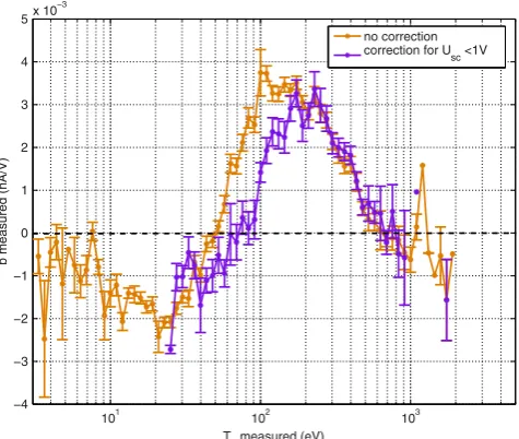
[50] Figure 4 shows such evidence for the Cassini LP. The slopeb measured is shown as a function of the elec-tron temperature of the ambient plasma measured by CAPS. The data set corresponds to the 2005–2008 LP measure-ments off the equator (|Z| > 2RS) and inside the secondary
electron current region (6.4 < L < 9.4), which implies that the b slope is essentially the bener contribution due to
energetic electrons. Two profiles are shown: corrected or not for the measurements with low spacecraft potentials (< 1V; see section 2.3.1.3). We added the profile not cor-rected for comparison: the statistics is better ( 40% more events) and except for the rare low electron temperature (i.e., few eV) events in our data set, the electron temper-ature measured should not be affected by including the low potentials.
Figure 4. Slope b (i.e., approximate bener given the data
selection) of the LP current-voltage curve as a function of the incident electron temperature Te measured by CAPS.
The data set corresponds to all data with6.4 < L < 9.4
and|Z| > 2RS between 1 February 2005 and 30 July 2008.
The CAPS data do either take into account (orange) or not (violet) the intervals with low spacecraft potential values (i.e.,Usc < 1V). The standard deviations are also shown for
[image:8.612.314.552.422.623.2][51] As will be developed in detail in section 5.1.3.1,bener
may be considered as proportional to
˛=
Z 1
0
E fie(E) (1 –ıe(E) –e(E))dE (8)
with fie(E) the incident electron distribution function at
energyE,ıe(E)the SEEY yield value, ande(E)the
back-scattering coefficient (see section 5.1.2 for further details). This quantity actually corresponds to the balance between the incident electrons and the secondary/backscattered elec-trons. Thus, the temperaturesTA andT*, where there is an
equilibrium between the incoming and the outgoing elec-trons (i.e., when˛= 0), also correspond to the temperatures wherebeneris null in the figure.
[52] Consequently, Figure 4 suggests that the critical and anticritical temperatures for the Cassini LP surface are, respectively, at600–800 eV and50–60 eV. These val-ues are in agreement with the broad range of valval-ues proposed
byLai and Tautz[2008] for a set of surface materials. As
shown in section 5.1.3.2, the energetic contributionIener to
the DC level of the current-voltage curve may also be con-sidered as proportional to the quantity˛and shows a similar curve (not shown) as a function of the electron temperature. The DC level is, however, less convenient to derive values forTAandT*.
[53] One can also infer from the bener = f(Te) profile
that the influence of the energetic electrons, though present for any incident electron temperature, will be maximum in the range [TA; T*], i.e., where the SEEY is maximum.
In the sections below, an additional criterion—beyond the criteria forL andZ values—on the incident electron tem-perature (e.g.,100 < Te < 500eV) will be used to select
appropriate time intervals for the modeling of the energetic electrons influence.
4. A First Approach to EstimateIenerandbener:
The Statistical Correlation With the 250–450 eV Electrons
[54] In this section, we will investigate a first method to reproduce the observed values ofIener/bener based on
statis-tical fits with the differential number flux of 253–474 eV electrons. We will deduce from this analysis to what extent the slopeb may be used to identify the regions where the energetic electrons have a strong impact.
4.1. A Statistical Analysis
[55] We showed in G12 and in section 3 above that theIener
andbener observations are correlated with the 253–474 eV
electrons, i.e., the peak energy of the SEEY function for the LP surface. We thus investigated this correlation further.
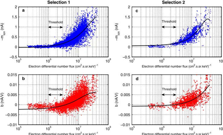
[56] Figure 5 shows these correlations with themionandb
values measured from 1 February 2005 to 30 July 2008, with two different selections among this large data set. Selec-tion 1 corresponds to the periods when the spacecraft was located off the equator at|Z| > 2RSand inside the secondary
electron current region in the L range 6.4–9.4RS (without
any criterion on the electron temperature). Selection 2 is a subselection of selection 1, with the CAPS-derived electron temperatures between 100 and 500 eV. The criteria used in these selections allow us to considermionandbas close to
the energetic DC level and slopeIenerandbenersince the
con-tribution of thermal ions should be small. Selection 2 focuses on the electron temperature range identified in section 3.2 as the range where the influence of the energetic electrons is the strongest.
[57] The best fit third-order polynomial functions are superimposed in each panel, with the following equations (xbeing the electron flux) and associated Pearson’s correla-tion coefficientsr[Press et al., 2007]:
[58] 1. Figure 5a:mion= –310–24x3+ 910–16x2– 7
10–8x+ 0.0336;r= 0.793.
[59] 2. Figure 5b:b= 210–25x3–210–17x2+710–10x–
0.0024;r= 0.578.
[60] 3. Figure 5c:mion = 310–23x3– 110–15x2– 4
10–8x– 0.0567;r= 0.802.
[61] 4. Figure 5d:b = –210–26x3+ 610–20x2+ 3
10–10x– 0.0008;r= 0.668.
[62] These results show a dispersion of the data, but the best fits functions provide a good estimation of mion and
b (i.e., Iener and bener given the selections criteria). The
estimation is better for the DC level than for the slope with respective correlation factors of0.8and0.6–0.65. Selecting the intervals with electron temperatures between 100 and 500 eV also ameliorates the correlation by about
0.1. This confirms again that these electrons are those which induce the largest energetic contributionsIenerandbener.
[63] The plots also allow to see a threshold effect, i.e., the existence of a minimum flux value for the incident elec-trons to influence the two parameters and start the increase observed. This threshold is approximately between 1 and
3106(keV cm2sr s)–1.
[64] The selections used above correspond to theLrange 6.4–9.4RS, where large 253–474 eV electron differential
number fluxes are often observed, but such energetic elec-trons are also present further in the magnetosphere. A statistical analysis (for the same data set) shows a decreas-ing occurrence of such large fluxes withL, but more than a third of the data show 253–474 eV fluxes above1106
(keV cm2sr s)–1atL= 16R
S. The data were selected in this
paper in order to reproduce accurately the influence of ener-getic electrons, but such an influence (though reduced) does exist in a large part of the Saturnian magnetosphere.
[65] One should add that the flux threshold observed cor-responds to the minimum flux to detect the influence of the energetic electrons given the data set considered, i.e., so that the energetic current is not masked by the ion cur-rent. Our data set selection allowed to remove most of the ion current contribution, so that the threshold values iden-tified are very close to the “real” threshold that would be observed in the total absence of ion contribution. However, if we changed our data set selection criteria to include data closer to the equator, allowing the presence of larger ion currents, the flux threshold would probably be observed at higher values.
4.2. The Slopebas a Criterion to Identify the Regions Influenced by the Energetic Electrons
GARNIER ET AL.: ENERGETIC ELECTRONS AND THE CASSINI LP
Figure 5. (a, c)–mion(i.e., approximate–Iener) and (b, d)bslope (i.e., approximatebener) values measured
by the LP as a function of the CAPS mean differential number flux of the 253–474 eV electrons. Two data sets are used here, corresponding to two selections of the data from 1 February 2005 to 30 July 2008. Selection 1 (in Figures 5a and 5b) corresponds to the data when the spacecraft was located off the equator at|Z| > 2RSand inside the secondary electron current region in theLrange 6.4–9.4RS. Selection 2
(in Figures 5c and 5d) is a subselection of selection 1, with the CAPS-derived electron temperatures between 100 and 500 eV. The solid black lines show the best fit third-order polynomial functions for each panel (see text for the equations used). The double arrows show the threshold flux values ([1 – 3]106
(keV cm2sr s)–1) above which the incident energetic electrons influence the–m
ionandbparameters.
[67] Figure 6 shows the occurrence, for the large data set, of positivebvalues as a function of the minimum 253– 474 eV electron differential number flux considered. The occurrence strongly increases when only large fluxes are selected, and goes beyond 50% above fluxes of 3106
(keV cm2sr s)–1up to values above 90%. Most of the slope
values are thus positive when the electron flux is beyond the flux threshold which induces the appearance of the energetic contributionsIener andbener(threshold identified in the
pre-vious section). However, there also exists positive values of beven for low electron fluxes (minimum20%). As a conse-quence, the only observation of positive slope values cannot be used as a criterion to identify the regions significantly influenced by the energetic electrons.
[68] Figure 7 shows the occurrence of electron fluxes above the flux threshold (three different values are consid-ered) as a function of the minimumb value. If we assume that the influence of the energetic electrons appears with fluxes larger than the threshold value, then large values of the slope may be a good criterion to identify such events. For example,80% of the data show electron fluxes above a threshold at1(respectively,3)106(keV cm2sr s)–1when
bis larger than2.1(respectively,2.8)10–3nA/V.
[69] The observation of large positive slope values may probably be used as a simple criterion during the LP analysis process to identify the regions where the energetic electrons have a significant influence. The limit b value to be used may be chosen depending on the probability wanted. The limit value may, however, be different in other environments (such as other magnetospheres than Saturn), whereas the
cri-terion over the electron temperature depends only on the probe surface composition.
4.3. Application to the Case Studies
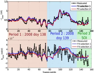
[70] The statistical analysis developed in section 4.1 was based on the large data set in order to obtain the best fit functions. Figure 8 shows the application of these fits to
[image:10.612.313.551.498.693.2]Figure 7. Probability of observing (253–474 eV) incident electron differential number fluxes above a certain thresh-old, as a function of thebvalue considered. Three different thresholds were considered (1/2/3106 (keV cm2sr s)–1),
leading to three probability curves.
the case studies, with a comparison between the observed and estimated values of the energetic DC level and slope of the current-voltage curve. One can derive the same conclu-sions as from the large data set analysis, i.e., selections 1 and 2 functions give similar good results, andIener is better
reproduced thanbener.
[71] The less good correlation for the slope is probably related to the noisy dynamics of the observedbvalue. The
slope of the current-voltage is indeed small in absolute value in such low-density plasma environments, which probably leads to a noisy profile. The different time intervals between the CAPS and LP data may also be an explanation for the less good correlation: the interpolation process may hide the high dynamics of the electron flux.
[72] We refer the reader to section 6 for a comparative dis-cussion on the precision of the various methods to reproduce the influence of the energetic electrons. The method using the 253–474 eV electron flux gives a good estimation of the Ienerandbenercontributions. It is, however, only an empirical
approach, with fit functions that cannot be applied directly to other plasma environments and that depend on the data set selection criteria used. As a consequence, one needs a more theoretical approach to understand further this influence.
5. A Second Approach: The Theoretical Influence of the Energetic Electrons
[73] In this section, we will use a theoretical approach to model the influence of the energetic electrons (incident, secondary, and backscattered), in order to reproduce the observedIenerandbenercontributions. We will first derive the
appropriate equations (section 5.1) before we compare with the observations (section 5.2) and infer the most appropriate maximum yield valueıemax(section 5.3) for the LP.
5.1. The Derivation of the Equations
[74] We will first determine the equation for the total current of incident/secondary/backscattered electrons at any bias voltage UB (section 5.1.1) before we detail the input
parameters needed (section 5.1.2) and infer the equations for Ienerandbener(section 5.1.3).
Figure 8. (top)–Ienerand (bottom)benermeasured (black) and estimated with the flux method fit
[image:11.612.142.470.442.698.2]GARNIER ET AL.: ENERGETIC ELECTRONS AND THE CASSINI LP
5.1.1. The Current Due to the Energetic Electrons [75] Modeling the exact current due to the energetic elec-trons is a very difficult task, due to the complex influence of several parameters: the influence of the floating poten-tial, of the sheath effects from the LP (due to a finite ratio between the sheath radius and the probe radius), the exact angular and energy distribution of the sedaries, etc. Consequently, several approximations are con-sidered in the literature to derive such equations, leading to several methods.
[76] Hastings and Garrett[1996] proposed equations for
the currents collected by a spacecraft for negative potentials. Assuming a Maxwellian distribution with a temperatureTse
for the secondaries, their approach leads to the following total current for incident and secondary electrons:
IHast= –
2e m2
e
ALP
Z 1
0 fie(E)
Z
0
sin()
(ıe(E,+/2)kBTse–E/2)ddE
(9)
with fie the incident electron distribution function, the
angle from the surface normal, andıe(E,+/2)the SEEY
energy and angular function.
[77] TheHastings and Garrett[1996] approach does take explicitly into account the secondary electron distribution function and the angular dependence of the SEEY but not the (repelling) effect of the surface potential on the incident electrons or sheath effects. However, several limitations pre-vent the use of this approach. First, the equation above was corrected for several errors existing inHastings and Garrett
[1996] (confirmed by D. Hastings, private communication): missing E and factor 2 in their equation 5.7, /2 miss-ing in equation 5.6. But beyond these errors, the quantity
ıe(E,+/2)kBTse–E/2in equation (9) will always be
neg-ative for energetic plasma environments (e.g.,Te > 10eV).
This equation thus corresponds to a negligible contribution of the secondaries in the total current collected. As a con-sequence, theHastings and Garrett[1996] approach cannot account for our observations.
[78] We chose as a first step the approach used byLai and
Tautz[2008], who proposed the following form for the total
(incident/secondary/backscattered) electron current (for U< 0):
ILai
Z 1
0
E fie(E) (1 –ıe(E) –e(E))dEe
eU
kBTe (10)
[79] This approach uses a simplified expression for the influence of the surface potential (through the Boltzmann termekBeUTe). Considering a corrected energyE–eUinstead
ofE for the secondary electrons would only slightly (by a few percent at maximum) change the results given the large electrons temperatures (hundreds of eV) and small potential values (a few volts). This approach provides a convenient analytical way to calculate the total current due to the ener-getic electrons. A normalization factor is, however, missing in equation (10) to derive the real current. Adding the nor-malization factor (by comparison with the expressions for spherical probes inMott-Smith and Langmuir[1926]) leads
to the final expression for the total currentIenergetdue to the
energetic electrons:
Ienerget=2e
m2
e
ALP
Z 1
0
E fie(E) (1 –ıe(E) –e(E))dE
*ekBeUTe (11)
[80] This total current Ienerget then impacts both the DC
level and slope of the LP current-voltage curve through the respective contributions Iener and bener, whose expressions
will be derived later.
5.1.2. The Choice of the Input Parameters
[81] The calculation of the current due to the energetic electronsIenergetneeds the knowledge of the incident electron
distribution functionfie(E)determined from the CAPS data
(see later in section 5.2), but it also needs the knowledge of both the secondary electron emission yield function (ıe(E);
see section 5.1.2.1) and the backscattering coefficient (e(E);
see section 5.1.2.2).
5.1.2.1. The Secondary Electron Emission Yield Function
[82] Several functional forms of the SEEY as a function the incident electron energy were used in our study:
[83] 1.Sternglass[1957]:ıe(E) = 7.4ıemax
E EMe
–2qE EM.
[84] 2.Lin and Joy [2005]: ıe(E) = 1.28ıemax
E EM
–0.67
1 –e–1.614EME 1.67
.
[85] 3.Sanders and Inouye[1978]:ıe(E) =c
e–aE–e –E
b
witha= 4.3EM,b= 0.367EMandc= 1.37ıemax.
with ıemax (maximum yield value) and EM (peak energy)
being free parameters to be determined for the LP surface composition. Theıemaxvalue will be chosen arbitrarily at first
in section 5.2. We will then propose a method to determine its best value and compare with laboratory measurements in section 5.3. The peak energyEMis chosen at350eV based
on G12.
[86] Figure 9 shows a comparison between the three pro-posed yield functions, assuming an arbitrary value ofıemax =
2. The yield byLin and Joy[2005] is the largest at high ener-gies and the smallest at low enerener-gies, whereas the function
bySternglass[1957] is the largest at low energies and close
toSanders and Inouye[1978] at high energies. The
influ-ence of the choice for the yield function is not significant as will be shown in section 5.2. A unique reference will be used,Sanders and Inouye[1978], since this yield curve is in between the two other references and its use is convenient for analytical integrations.
5.1.2.2. The Electron Backscattering Coefficient [87] The backscattering electrons are mostly significant at low incident energies (few eV). A backscattering coeffi-cient may be, however, included for detailed calculations. This coefficient depends on the exact surface composition, the incident electron energy, or the incidence angle of these electrons. Monte Carlo simulations (M. Belhadj, French Aerospace Laboratory, private communication) for TiN sur-faces givee(E)0.2–0.4. We thus choose as a first step a
constant backscattering coefficient at0.3.
[88] Moreover, the secondary and backscattered electrons shall be considered together (e+ıein the equations). Insofar
Figure 9. Comparison between three different secondary electron emission yield functions as a function of the energy of the incident electrons. The peak energyEM is defined at
350 eV based on Garnier et al. [2012b], and an arbitrary value of2was chosen for the maximum yieldıemax.
the precise value of the constante(E)value has no
signifi-cant influence: a slight change ine(E)corresponds directly
to a slightly different value forıemax.
5.1.3. The Equations for the Energetic Electrons ContributionsbenerandIener
5.1.3.1. ThebenerContribution
[89] Thebslope of the current-voltage curve is defined by equation (7). Consequently, thebenercontribution due to the
energetic electrons is similarly given by
bener= –
Ienerget(UB= –5 V) –Ienerget(UB= –32 V)
–5 + 32 (12)
Combining with equation (11) forIenergetleads to
bener= –
2e m2
e
ALP(
Z 1
0
E fie(E) (1 –ıe(E) –e(E))dE)
*e e(Vfloat –5)
kBTe –e e(Vfloat –32)
kBTe
32 – 5
(13)
which can be written as
bener= – I0A
27 (14)
with
I0=
2e m2
e
ALP(
Z 1
0
E fie(E)(1 –ıe(E) –e(E))dE) (15)
and (sinhhyperbolic sinus function)
A=e e(Vfloat –5)
kBTe –e e(Vfloat –32)
kBTe (16)
= 2e e(Vfloat –37/2)
kBTe sinh ( 27e 2kBTe
) (17)
[90] The integralI0will then be calculated with two
meth-ods: (1) using the full electron distribution measured by CAPS ELS or (2) assuming a Maxwellian distribution and using the electron momentsne andTeprovided by the same
instrument (see section 2.3.1 for more details about the CAPS ELS data).
[91] If we choose the full measured distribution, we have first to transform the initial differential number fluxesF(E)
((keV cm2sr s)–1) measured in each of the 64 energy
chan-nels into the distribution functionfie(s3m–6):
fie(E)
5m2
eF(E)
eE (18)
[92] The integral I0 is then calculated numerically from
the knowledge of the differential number fluxes measured by CAPS ELS.
[93] If we choose the method based on the electron momentsneandTe, as well as the SEEY function bySanders
and Inouye[1978], then the integral I0 may be calculated
analytically (see Appendix A):
I0=neKL (19)
with
K=
s
kBTe
2me
ALPe (20)
L= 1 –e+
cb2
(b+kBTe)2
– ca
2
(a+kBTe)2
(21)
[94] The final expressions forbener are, respectively, for
the full ELS distribution and a Maxwellian distribution: (
benerfull = –10ALPA 27
R1
0 F(E)(1 –ıe(E) –e(E))dE benermaxw = –AneKL
27
(22)
5.1.3.2. TheIenerContribution
[95] The initial DC levelmof the current-voltage curve is defined by
m=
RUB= –32
UB= –5 (I–(UB) +bUB)dUB
27 (23)
[96] TheIenercontribution to the DC level of the
current-voltage curve of the LP is thus given by
Iener=
RUB= –5
UB= –32(Ienerget(UB) +benerUB)dUB
27 (24)
which leads to
Iener= I0
RUB= –5
UB= –32(e e(Vfloat +UB )
kBTe –AUB/27)dUB
27 (25)
leading, using the parametersI0andA, to
Iener=
AI0(kBeTe – 37/2)
27 (26)
[97] The calculation of I0 (see previous section and
Appendix A) gives the following final expressions forIener,
respectively, for the full ELS distribution and a Maxwellian distribution:
8 < :
Ienerfull = –
10ALPA(kBeTe–37/2) 27
R1
0 F(E)(1 –ıe(E) –e(E))dE
Ienermaxw =
AneKL(kBeTe–37/2) 27
GARNIER ET AL.: ENERGETIC ELECTRONS AND THE CASSINI LP
Figure 10. (top)–Ienerand (bottom)benermeasured and modeled with the full distribution method during
the case studies (inbound and outbound legs of the high-inclination orbit, SOI). The modeled values use several SEEY functions [Sternglass, 1957;Lin and Joy, 2005;Sanders and Inouye, 1978] as well sev-eral levels of simplifications for the expressions ofIener/bener(“simpl1”/“simpl2” refer to the first/second
simplification level). See the text for more details.
5.1.3.3. Simplified Expressions
[98] The expressions for bener andIener developed in the
previous sections need the knowledge of several informa-tion: the electron distribution (in particular the electron temperatureTederived after a complex analysis of the CAPS
ELS data), the secondary and backscattering coefficients, and also the floating potentialVfloat.Vfloatis derived from an
independent and nonautomatic analysis of the electron side (positive potentialU) of the LP current-voltage curve.
[99] If we want to remove the parasite contribution due to the energetic electrons from the LP observations dur-ing the Cassini mission, the search of easy and automatic calculations should be investigated. Two levels of simplifi-cation may be used to derive expressions needing less input parameters.
[100] If we focus on the regions where the electron tem-perature is large, and given the low absolute values of the potentialVfloat (e.g.,–1.1 < Vfloat < +0.5V during the case
studies), the expression of the parameterAmay be simplified to removeVfloat. For low ratios e(Vfloatk –37/2)
BTe , we have A 27e
kBTe
(28)
[101] One then directly replacesAby this approximation into the equations forbener (22) andIener (27) to obtain the
simplified parameters benersim and Ienersim where Vfloat is not
present anymore.
[102] A second level of simplification can be applied to the calculation ofIener in order to remove both the electron
temperature and the floating potential. If we again con-sider large enough temperatures, the ratio
kBTe e –37/2
kBTe e
! 1,
so that equation (26) (combined with equation (28)) simply becomes
IenerIenersimpl2=I0 (29)
[103] This simplification allows, when using the full measured distribution instead of the electron moments, to approximateIener with the only use of the CAPS ELS flux
distribution measured.
[104] The first approximation induces an error between
4.0/3.7% and21.3/19.4% forVfloatbetween–1.1and+0.5V
and forTe = 100/500eV. The second simplification induces
in the end an error of49/21/8% forTe= 100/200/500eV and
|Vfloat| < 1V.
[105] The influence of the simplification levels will be discussed in the next section and shown in Figures 10 and 11. In the absence of additional information, the exact expressions were always used in the paper to obtain more rigorous results.
5.2. Comparison With the Observations During the Case Studies
[106] In this section, we will compare the modeled and measured Iener andbener contributions during the case
studies by using maximum yield values derived later in section 5.3.1.
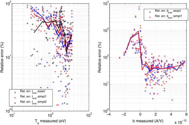
[107] Figure 10 shows the resulting comparison between the modeled and measured values ofIener andbener for the
full distribution method (defined in section 2.3.1.1). The maximum yield valuesıemaxused for both parameters were,
Figure 11. (top) –Iener and (bottom) bener measured and modeled with the moments method during
the case studies (inbound and outbound legs of the high-inclination orbit, SOI). Several levels of sim-plification for the expressions of Iener/bener are compared (“simpl1”/“simpl2” refer to the first/second
simplification level). See the text for more details.
i.e., two levels of simplification forIener and one forbener.
Moreover, the influence of the choice of the SEEY function is shown, with a comparison between the three references detailed in section 5.1.2.1.
[108] The relative errors (after a quartile filtering) between the measured and modeled parameters are of the same order for any yield function or simplification level:
27–33% forIenerand53–62% forbener. There is a few
percent increased error for simplified expressions compared with the exact formula and a minimum error for the yield function given bySanders and Inouye[1978]. Moreover, the DC level is better reproduced than the slope of the current-voltage curve due to the dynamic profile of the measured slope (as discussed in section 4.3).
[109] Figure 11 shows the same comparison for the moments method (defined in section 2.3.1.3). The
maxi-mum yield values ıemax used were 1.3 and 1.15,
respec-tively, for Iener and bener (see section 5.3.1 and Table 1).
The figure shows the modeled parameters for several lev-els of simplifications and the Sanders and Inouye [1978] SEEY function.
[110] The relative errors (after a quartile filtering) are of the same order as for the full distribution method, though slightly enhanced, with36–40% forIenerand57–63%
forbener. The exact expressions and the DC level still give
the best results.
[111] The two figures, however, show significant errors at some time intervals of the case studies. In particular, the full distribution method is not always efficient during periods 2 and 3, and the moments method is not appropriate during the beginning of period 2 and during a part of period 3. These large errors may be explained by two main problems. First,
Table 1. Comparison Between the Different Methods to Reproduce theIenerandbenerContributions During the Case Studiesa
Rel. error Rel. error Rel. error all
Inb. (%) ıemaxInb. Inb.-Outb. (%) ıemaxInb.-Outb. periods (%) ıemaxall periods
Iener
Statistical method selection 1 14/12 n/a 14/13 n/a 16/15 n/a Statistical method selection 2 13/12 n/a 13/13 n/a 15/14 n/a Full CAPS ELS distribution 18/16 3.65/3.75 21/20 3.6/3.6 27/25 3.6/3.6
Electron moments 39/38 1.3/1.3 33/33 1.3/1.3 36/26 1.3/1.3
bener
Statistical method selection 1 49/69 n/a 57/75 n/a 66/80 n/a Statistical method selection 2 47/59 n/a 54/63 n/a 60/72 n/a Full CAPS ELS distribution 40/53 3.45/3 44/55 3.25/3 55/62 3.2/3 Electron moments 49/58 1.15/1.1 53/65 1.15/1.1 58/77 1.15/1.1
aThe statistical method (section 4.1) uses fit functions based on the analysis of two initial different data selections (shown in Figure 5) whereas the theoretical approach (section 5.1.3) uses either the full electron distribution measured or the derived electron moments. The relative errors between the measurements and modeling are given in percent after a quartile filtering. The best values for the maximum yield
[image:15.612.78.535.553.675.2]