Proportional integral plus control applications of state dependent parameter models

Proportional-integral-plus control applications

of state-dependent parameter models

C J Taylor1*, E M Shaban1, M A Stables1,andS Ako2

1Engineering Department, Lancaster University, Lancaster, UK

2Bachy Soletanche Limited, Burscough, UK

The manuscript was received on 10 October 2006 and was accepted after revision for publication on 23 May 2007.

DOI: 10.1243/09596518JSCE366

Abstract: This paper considers proportional-integral-plus (PIP) control of non-linear systems defined by state-dependent parameter models, with particular emphasis on three practical demonstrators: a microclimate test chamber, a 1/5th-scale laboratory representation of an intelligent excavator, and a full-scale (commercial) vibrolance system used for ground improve-ment on a construction site. In each case, the system is represented using a quasi-linear state-dependent parameter (SDP) model structure, in which the parameters are functionally dependent on other variables in the system. The approach yields novel SDP–PIP control algorithms with improved performance and robustness in comparison with conventional linear PIP control. In particular, the new approach better handles the large disturbances and other non-linearities typical in the application areas considered.

Keywords: control system design, non-minimal state space, state-dependent parameters, hydraulic actuators, system identification

1 INTRODUCTION but with additional dynamic feedback and input

compensators introduced automatically when the process has second-order or higher dynamics, or Previous papers have considered the

proportional-pure time delays greater than unity. In contrast to integral-plus (PIP) controller, in which non-minimal

conventional PI/PID control, however, PIP design state-space (NMSS) models are formulated so that full

exploits state variable feedback (SVF) methods, where state variable feedback control can be implemented

the vagaries of manual tuning are replaced by pole directly from the measured input and output signals

assignment or linear quadratic (LQ) design. of the controlled process, without resort to the

To date, however, inherent non-linearities in the PIP design and implementation of a deterministic state

system have been accounted for in a rather ad hoc reconstructor (observer) or a stochastic Kalman

manner at the design stage, sometimes leading to filter [1–3].

reduced control performance. For example, pressure Such PIP control systems have been successfully

disturbances sometimes take the ventilation rate in a employed in a range of practical applications,

parti-building sufficiently far from the operating condition cularly in the areas of microclimate control for

on which the linear controller is based for the agricultural buildings [4,5], and in the automation

response to such a disturbance to be relatively slow. of construction robots on building sites [6,7]. In both

Similarly, on a construction site, the behaviour of these application areas, the most common types of

hydraulically driven manipulators is dominated by controller used previously have been derived from

the highly non-linear, lightly damped dynamics of the ubiquitous proportional-integral-derivative (PID)

the actuators [10]. approach (see, for example, references [8] and [9]).

To improve PIP control in such cases, therefore, In this regard, PIP control can be interpreted as one

the present paper identifies, and subsequently exploits logical extension of conventional PI/PID methods,

e.g. Young [11]. The linear-like, affine structure of the 2.1 Model structure SDP model means that, at each sampling instant, it

Consider the deterministic form of the SDP model can be considered as a ‘frozen’ linear system. This _[11,16]

formulation may then be used to design an SDP–PIP

y

k=wTkpk (1)

control law at each sampling instant using linear

methods [12]. _{where wT}

k is a vector of lagged input and output The present paper develops this new approach for _{variables and p}

k is a vector of SDP parameters, three practical demonstrators, related to both the _{defined as follows}

above application areas: a microclimate test chamber

wT

k=[−yk−1 −yk−2 , −yk−n uk−1 , uk−m] representing a section of a livestock building, a

1/5th-scale laboratory model of an intelligent excavator, p

k=[a1{xk} a2{xk} , an{xk} b1{xk} , bm{xk}]T and a full-scale (commercial) vibrolance system used _Here,

y

kis the output andukthe control input, while for ground improvement on a construction site.

a

i{xk} (i=1, 2, … ,n) and bj{xk} (j=1, … , m) are With regard to the first of these examples, the

state-dependent parameters. The latter are assumed paper focuses on the control of ventilation rate using _{to be functions of a non-minimal state vector} an axial fan. Ventilation is one of the most significant

xT

k=[wkT Uk] in which Uk=[U1,k, U2,k, … , Ur,k] is a inputs in the control of the microclimate surrounding _{vector of other variables, not necessarily y}

k or uk. plants or animals within the majority of agricultural _{However, for SDP–PIP control system design, it is} buildings [13]. For example, without adequate fresh _{usually sufficient to limit model (1) to the case where} air supply within a livestock enclosure, animal com- _xT

k=wTk. Any pure time delay t1 is represented fort and welfare are drastically reduced, especially _{by setting the leading b}

1{xk} …bt−1{xk} terms to during high-density occupation, where excessive levels _{zero. Finally,n and mare integers representing the} of moisture, heat, and internal gases are generated. _{maximum lag associated with the output and input}

By contrast, in the civil and construction industries, _{variables respectively.}

semi-automatic functions are starting to be adopted _{Numerous recent publications describe an approach} as a means of improving efficiency, quality, and safety. _{for the identification and estimation of the SDP model} The control problem is made difficult by a range of _{defined by equation (1), together with the application} factors that include highly varying loads, speeds, and _{of such methods to a wide range of environmental,} geometries, as well as the soil–tool interaction in the _{biological, and engineering systems (see references} case of autonomous excavators [14,15]. In the pre- _{[11] and [16] and the references therein). In the} sent paper, inverse kinematics is utilized online to _{present context, the approach is broadly composed} convert the task into a desired trajectory in the joint _{of two distinct stages, as discussed below.}

space, while a feedback controller regulates the

2.2 Model identification applied voltage to the hydraulics, so as to maintain

these joint angles.

The underlying model structure and potential state In each case, the novel SDP–PIP approach is com- _{variables are first identified by statistical estimation} pared with a benchmark linear PIP design. Sections _{of discrete-time linear transfer function models. Such} 2 and 3 of the paper describe the identification and _{models take a similar form to equation (1) but with} control methodologies. Sections 4 to 6 introduce _{time-invariant parameters, i.e.a}

i(i=1, 2, … , n) and each demonstrator and present the implementation _b

j (j=1, … , m) are constant coefficients, estimated results. Finally, the conclusions are given in section 7. _{using the simplified refined instrumental variable}

(SRIV) algorithm [17,18].

Two main statistical measures are utilized to help identify the most appropriate linear model structure, 2 SYSTEM IDENTIFICATION i.e. the values ofnandmand the time delayt. These

are the coefficient of determinationR2

T,based on the

The controllers used in this paper are based on the response error, and Young’s identification criterion, simplest multiple-loop, single-input, single-output which provides a combined measure of model fit and models. In the case of the robot arms, there is some parametric efficiency [17,18].

However, since the changes in the parameters are initial conditions for the optimization are based on the SDP estimates obtained from the earlier KF/FIS functions of the state variables, the system may

stage of the analysis. This helps to avoid the potential exhibit severe non-linear or even chaotic behaviour.

problem of fminsearch finding a local (rather than Normally, this cannot be approximated in a simple

global) optimal set of parameters. TVP manner because the parameters can vary at a

very rapid rate. For this reason, recourse is made to a novel approach that again exploits recursive KF/FIS estimation but this time within an iterative

3 CONTROL METHODOLOGY ‘backfitting’ algorithm that involves special reordering

of the time series data [11,16].

The NMSS representation of system (1) is

x

k+1=Fkxk+gkuk+dyd,k 2.3 Parameter estimation

y k=hxk Eacha

i{xk} andbj{xk} in model (1) can be considered (2)

as a ‘non-parametric’ estimate because it has a

different value at each sample and can only be _{where the non-minimal state vector at the kth} viewed in complete form as a graph. However, it is _{sample is defined as}

possible to proceed to a final parametric estimation

stage where the non-parametrically defined non- x

k=[yk , yk−n+1 uk−1 , uk−m+1 zk]T linearities obtained initially by KF/FIS estimation are

and z

k=zk−1+[yd,k−yk] is the integral of error now parameterized in some manner in terms of their

between the reference or command input y d,k and associated dependent variable.

the sampled output y

k. As usual for NMSS design, This can be achieved by defining an appropriate

inherent type 1 servomechanism performance is parametric model in some convenient form, such

introduced by means of this integral-of-error state [1]. as a trigonometric function, a radial basis function,

The state transition matrixF_kand input vectorg_k at or a neural network. The parameters of this

para-the kth sample, together with the time-invariant meterized model can then be estimated directly

commanddand observation vectors h, are defined from the input–output data using some method of

as follows dynamic model optimization, e.g. deterministic

non-linear least squares or a more statistically efficient

F

k=[F1,k F2,k] stochastic method, such as maximum likelihood.

However, for the practical applications considered _g

k=[b1{xk+1} 0 0 , 0 1 0 , 0 −b1{xk+1}]T below, polynomial or linear functions of the state

variables are sufficient for control system design. The d=[0 0 0 , 0 1]T associated coefficients are straightforward to estimate

h=[1 0 0 , 0 0] using standard numerical optimization functions,

such as fminsearch in MATLABA. In this case, the

with the components

F 1,k= t N N N N N N N N N N N N N N N v −a

1{xk+1} −a2{xk+1} , −an−1{xk+1} −an{xk+1}

1 0 , 0 0

0 1 , 0 0

e e P e e

0 0 , 1 0

0 0 , 0 0

0 0 , 0 0

e e P e e

0 0 , 0 0

a

F_2,k= t N N N N N N N N N N N N N N N v

b₂{x

k+1} , bm−1{xk+1} bm{xk+1} 0

0 0 0 0 0

0 0 0 0 0

e e e e 0

0 , 0 0 0

0 , 0 0 0

1 , 0 0 0

e P e e e

0 , 1 0 0

−b₂{x

k+1} , −bm−1{xk+1} −bm{xk+1} 1 u N N N N N N N N N N N N N N N w

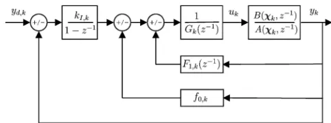
Fig. 1 SDP–PIP control implemented in feedback form

A(x_k, z−1) and B(x_k,z−1) in Fig. 1 represent the SDP model (1) in polynomial form, similar to a transfer function but with state-dependent parameters [11,16].

Note that the elements of the (n+1)th row ofF kare

all zero ifm>1. _{3.2 Controllability}

A prerequisite of global controllability is that the 3.1 Control algorithm

system {F

k,gk,h,d} is piecewise controllable at each The control law takes the usual SVF form _{sample k, with the standard NMSS controllability} conditions applying over the sampling period. This

v

k=−lkxk (3) _{requirement follows from the fact that, if a system}

where the control gain vector _{is globally controllable, it clearly has to be locally} controllable. Although omitted here for brevity,

l

k=[f0,k , fn−1,k g1,k , gm−1,k −kI,k} such NMSS/PIP linear controllability conditions are derived by Younget al.[1].

is obtained at each sampling instant by either pole

assignment or optimization of an LQ cost function. The first condition states that there should be no pole zero cancellations in the model, while the With regard to the latter approach, earlier research has

either used a ‘frozen-parameter’ system defined as a second avoids the presence of a zero at unity, which would cancel with the unity pole associated with sample member of the family of NMSS models

{F

k,gk,d,h} or has solved the discrete-time algebraic the integral action. In the SDP–PIP case, it is straight-forward to check these conditions at every sampling Riccatti equation at each sampling instant [12]. For

pole assignment, the control gains are similarly deter- instant to ensure local controllability. If they fail to hold at thekth sample, model (1) is instead evaluated mined using linear methods. One approach, for

example, involves definition of a genericSmatrix [1]. for k−1. Unfortunately, this effectively leaves the system in linear (fixed-gain) mode for a period of Alternatively, it is straightforward to derive algebraic

solutions for specific cases, as illustrated in reference time, something that can be undesirable in practice. For this reason, the present research first identifies [21].

Note that the expected design response in the pole any problem regions of the parameter space by off -line simulation. This is feasible because, in practice, assignment case, such as dead-beat or a specified

degree of overshoot, is only obtained when the most the system variables will always be constrained to lie within a certain range. For example, the boom angle recent SDP estimates are utilized, i.e. F_k and g_k are

defined in terms of x

k+1 rather than xk in equations of the vibrolance system is limited by hardware to 060°, while the input is a voltage signal scaled (2). This result mirrors that found for PIP control of

bilinear systems, a special case of the SDP model con- within ±1000 (section 6). The trajectory of the command input is subsequently chosen to avoid sidered here [22]. In a similar manner to the present

example, reference [23] demonstrates that the bilinear local controllability problems, if any arise. Of course, such an approach is necessarily based on a case-parameter utilized in the control law should be based

onk+1 rather than k. by-case empirical study and, as the order of the

system increases (for example with multiple state Figure 1 illustrates the SDP–PIP controller in block

diagram form, where the control polynomials are dependencies), requires an increasing computational burden to evaluate [24].

given by F

1,k(z−1)=f1,k+,+fn−1,k and Gk(z−1)= 1+g

of ongoing research by the authors, the pragmatic approach described above appears satisfactory for all three applications considered in the present paper, as shown below.

4 VENTILATION CHAMBER

Taylor [25] describes the utility of a 2 m2 by 1 m forced-ventilation test chamber at Lancaster University. A computer-controlled axial fan is positioned at the outlet in order to draw air through the chamber, while an air velocity transducer measures the associated ventilation. The inlet airflow is independently regulated by a second fan, utilized to represent realistic pressure disturbances and

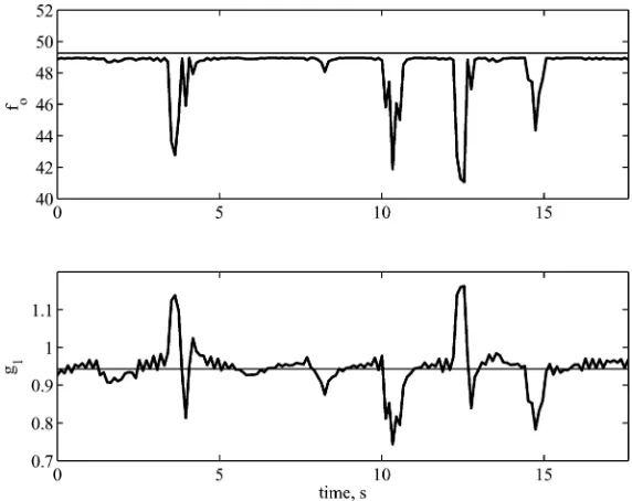
Fig. 2 Ventilation rate SDP model. Upper graph:a

1{xk} external wind conditions. _{estimates (dots) and least-squares fitted straight} line (solid trace) plotted against air velocity 4.1 SDP model for ventilation rate _{(m/s). Lower graph: power curve represented} by equation (5), showing the steady-state air Analysis of experimental data from the chamber

velocity (m/s) plotted against the scaled voltage yields the following SDP model for ventilation rate, _{input (%)}

witht=2sample time delays [21] y

k=−a1{xk}yk−1+b2{xk}uk−2

For comparison, a fixed-gain PIP controller is also a

1{xk}=a1+a2yk−1 developed for an operating level of 4–5 m/s. As would be expected, the performance of the SDP–PIP and b

2{xk}= w{u

k−2}(1+a1{yk−1}) u

k−2 linear PIP designs are very similar for ventilation

rates close to this operating level. (4)

By contrast, Fig. 3 shows the advantage of the where a

1 anda2 are constant coefficients,w{uk−2} is non-linear approach when low airflow rates are the non-linear relationship discussed below,y

kis the encountered (similar results emerge for high airflows). outlet air velocity (m/s), andu

kis the voltage applied to the fan, expressed as a percentage of the maximum voltage. Equation (4) is based on a sampling rate of 2 s, which yields a good compromise between a fast response and a desirable low-order model.

At high applied voltages, the steady state airflow rate converges asymptotically to a maximum value determined by the characteristics of the fan, defined by the following relationship based on a logistic growth function

y

2=w{u2}=

G

max

1+e−h(u₂−x₀)1/c

H

where y

2 is the steady-state air velocity, u2 is a constant applied voltage, and y

max, h, x0, and c are

coefficients. Figure 2 illustrates the estimated linear state dependency for a

1{xk} and the power curve equation (5).

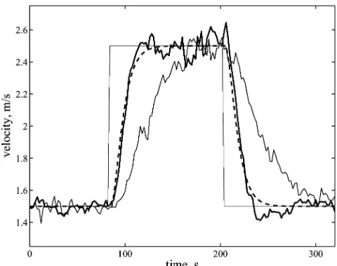
Fig. 3 Ventilation chamber implementation experiment showing the air velocity plotted against time (s): 4.2 Implementation

command input (step changes), SDP–PIP (thick For the present example, SDP–PIP design is based trace), fixed-gain PIP (thin), and simulated

Figure 3 shows that the SDP–PIP-controlled output 5 LABORATORY EXCAVATOR approximates the desired speed of response specified

by the pole positions, determined by simulating the The laboratory robot arm is a 1/5th-scale represent-ation of the more widely known Lancaster University design polynomial in open loop. By contrast, the

inherent model mismatch of the linear controller computerized intelligent excavator (LUCIE), which has been developed to dig trenches on a construction yields a significantly slower response.

In the context of agricultural buildings, the site [6,9]. It provides a valuable test bed for the safe development of new control strategies before disturbance response illustrated by Fig. 4 is of

parti-cular significance. Here, the secondary fan at the implementation on full-scale systems.

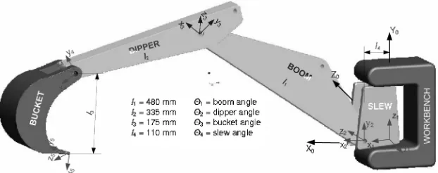
As illustrated in Fig. 5, the arm consists of four chamber inlet is employed to simulate large pressure

disturbances. These disturbances temporarily take hydraulically actuated joints. The joint angles are measured directly by mounting rotary potentiometers the ventilation rate away from the operating level of

the fixed-gain controller, and hence the SDP–PIP concentrically with each joint pivot. These signals are routed to high-linearity instrumentation amplifiers design reacts fastest to the problem.

within the card rack for conditioning before forward-ing to the A/D converter. The rig is supported by multiple I/O asynchronous real-time control systems, which allow for multitasking processes via modularization of code written in Turbo C++A.

Valve calibration is based on normalizing the input voltage of each joint into input demands, which range from −1000 for the highest possible downward velocity to+1000 for the highest possible upward velocity. Here, an input demand of zero corresponds to no movement. Note that, without such valve calibration, the arm will gradually slack down because of the payload carried by each joint (see reference [24] for details).

In open-loop mode, the arm is manually driven to dig a trench in the sandpit, with the operator using two analogue joysticks, each with two degrees of freedom. The first joystick is used to drive the boom Fig. 4 Ventilation chamber disturbance experiment. _{and slew joints, while the other is used to move the} Upper graph: air velocity with the operating _{dipper and bucket joints. In this manner, a skilful} level removed, plotted against time (s):

com-operator moves the four joints simultaneously to mand input (constant), SDP–PIP (thick trace),

perform the task. By contrast, the objective here is to and fixed-gain PIP (thin). Lower graph: SDP–PIP

design a computer-controlled system for automatic control input (thick) and disturbance fan input

(thin), both scaled voltages (%) digging without human intervention.

5.1 Kinematics invariant parameters. Note that the arm essentially acts as an integrator, since the normalized voltage The kinematic equations below allow the tool tip to

has been calibrated so that there is no movement be programmed to follow the planned trajectory, while

whenu

k=0. In fact, a1=−1 is fixed a prioriin the

the bucket angle is separately adjusted to collect or

final model, so that only the numerator parameter release sand. In this regard, Fig. 5 shows the laboratory

b

tis estimated in practice for linear PIP design. excavator and its dimensions, i.e.h

i(joint angles) and However, further analysis of open-loop data reveals l

i(link lengths), wherei=1, 2, 3, and 4 for the boom, limitations in the linear model. In particular, the dipper, bucket, and slew respectively.

value of b

t changes by a factor of ten or more, Given {X, Y, Z} from the trajectory planning routine,

depending on the applied voltage used in the step i.e. the position of the end-effector using a

coordi-experiments. In fact, SDP analysis suggests that a nate system originating at the workbench, together

more appropriate model for the boom takes the form with the orientation of the bucket H=h

1+h2+h3, of equation (4) with the following inverse kinematic algorithm is derived

by Shaban [24] using the well-known Denavit– a

1{xk}=0.28×10−6u2k−2−1 Hartenberg convention. Here,C

iandSidenote cos(hi) _b

2{xk}=−5.8×10−6uk−2+0.0194 and sin(h

i) respectively, whileC123=cos(h1+h2+h3)

(12) h

4=−arctan

C

X

D

compared with typical open-loop data for the boom. X₉=X−l4C4

C 4

−l

3C123 (7) Here, the input sequence consists of a random series of step inputs at random levels, so as to fully excite Y₉=Y−l

3S123 (8) the non-linearities in the system. For this reason,

only the SDP model captures the dynamic behaviour of the system (R2_T=0.9), while the SRIV estimated h

1=arctan

C

1+l2C2)Y9−l2S2X9 (l

1+l2C2)X9−l2S2Y9

D

(9)

linear model fails to converge to a useful solution (R2

T<0).

h

2=±arccos

C

X₉2+Y₉2−l2 1−l22 2l

1l2

D

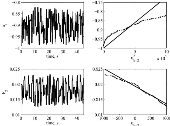
(10) _{Finally, Fig. 7 illustrates the parameter estimates} associated with equation (12). The unsorted time h

3=H−h1−h2 (11) histories of each SDP are shown on the left-hand subplots, while the right-hand subplots illustrate the During the excavation of a trench, each cycle can

more meaningful state dependencies. For brevity, be divided into four distinct stages: positioning the

similar SDP models for the dipper, slew, and bucket bucket to penetrate the soil; the digging process in

angles are omitted here. However, full details of these a horizontal straight line along the specified void

models and associated SDP–PIP control algorithms length; picking up the collected sand from the void to

are reported by Shaban [24]. In this case, the control the discharge side; and discharging the sand. For the

algorithms are updated at each sampling instant present example, the speed profile typically ramps

using linear LQ methods. up at a constant acceleration before proceeding at a

constant speed and finally ramping down to zero at

5.3 Implementation a constant deceleration [24].

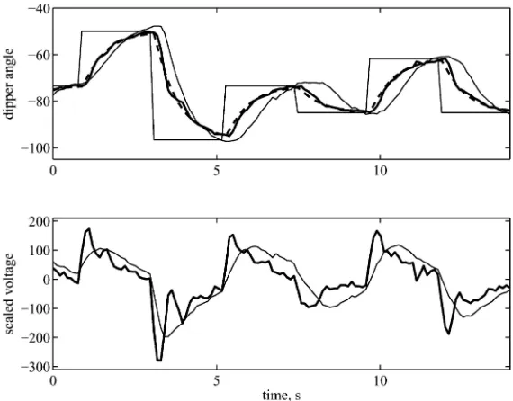
Typical implementation results for the boom arm 5.2 SDP models for joint angle

are illustrated in Fig. 8, where it is clear that the SDP–PIP algorithm is more robust than the linear For linear PIP design, open-loop step experiments

are first conducted for a range of applied voltages PIP algorithm to large steps in the command level. In fact, the linear design yields unwelcome high-and initial conditions, all based on a sampling rate

of 0.11 s. In this case, the SRIV algorithm suggests frequency oscillations in the control input signal. Note that the two controllers are designed to yield a that a first-order linear model witht samples time

delay, i.e. y

k=a1yk−1+btuk−t provides an approxi- similar speed of response to the theoretical case, shown as the dashed trace, and hence the differences mate representation of each joint, witht=1 for the

dipper and bucket joints and t=2 for the boom seen in Fig. 8 are entirely due to the inherent non-linearities in the system. The time-varying SDP–PIP and slew.

Here, y

k is the joint angle and uk is the scaled control gains for this experiment are compared with the linear gains in Fig. 9.

voltage in the range±1000, while {a

time-Fig. 6 Open-loop data for the laboratory excavator boom arm. Upper graph: boom angle (deg, dots) and SDP model response (solid) plotted against time (s). Lower graph: scaled input voltage

Fig. 7 Parameter estimates for the laboratory excavator boom arm. Left-hand graphs: SDP estimates plotted against time (s). Right-hand graphs: SDP estimates plotted against state variable, showing a typical realization from one experiment (dots) and the optimized fit from four datasets (solid)

It should be pointed out that the response time in this case, even small variations in the response time are multiplied up when the bucket position is for this example has been deliberately increased to

the practical limit of stable linear PIP control in order finally resolved in the sandpit.

In the latter regard, Table 1 compares the response to emphasize these differences. By contrast, Fig. 10

illustrates control of the dipper arm using slower time of the PIP and SDP–PIP approaches, represented by the number of seconds taken to complete three LQ weightings. Here, the SDP–PIP response closely

follows the theoretical design response, while the complete trenches, each consisting of nine digging cycles. Here, the improved joint angle control allows linear controller is rather slower. Although the

Fig. 8 Isolated control of the laboratory excavator boom arm, using relatively ‘fast’ control weights. Upper graph: command input (deg, sequence of step changes), theoretical response (dashed), non-linear SDP–PIP (thick), and linear PIP (thin), plotted against time (s). Lower graph: scaled input voltages

Fig. 9 Non-linear SDP–PIP (thick) and linear PIP (thin) control gains for the experiment shown in Fig. 8, plotted against time (s). Upper graph: proportional gain. Lower graph: input gain

per cent reduction in the digging time. Finally, Fig. 11 Table 1 Time (s) taken to complete

illustrates typical SDP–PIP implementation results for one trench

one cycle of the bucket, showing a three-dimensional Trench SDP–PIP Linear PIP _{coordinate plot of the end-effector. This graph} shows the bucket being first lowered into and sub-1 339 369

2 334 370 _{sequently being dragged through the sand, followed}

3 336 373

Fig. 10 Isolated control of the laboratory excavator dipper arm. Upper graph: command input (deg, sequence of step changes), theoretical response (dashed), non-linear SDP–PIP (thick), and linear PIP (thin), plotted against time (s). Lower graph: scaled input voltages

Fig. 11 Resolved position of the laboratory excavator end-effector for one digging cycle in sand using SDP–PIP control, showing the planar horizontal and vertical displacements (XandZ), together with the slewY, with the setpoint shown as straight lines (mm)

6 GROUND COMPACTION lowered into the ground, penetrating downwards by regulating the boom (joint 2) and dipper (joint 3).

Here, the objective is to keep the arm tip moving With regard to the full-scale commercial system, the

field tests utilized a KOMATSU-PC-240-LC-7 hydraulic in a vertical straight-line path. In this manner, the surrounding soil is compacted up to a distance of excavator, as illustrated in Fig. 12. The vibrolance is

connected to the excavator arm and hangs freely like about 5 m from the probe; for granular soils, the cavity produced is subsequently filled with gravel. a pendulum (joint 4). The operator first positions the

follows

b

b{xk}=1.5×10−11u3k−2+1.3×10−9u2k−2 −1.88×10−5u

k−2+0.007 (13) The equivalent model for the dipper has

b

d{xk}=−1.078×10−5|uk−2|+0.015 (14) where |u

k−2| represents the absolute value of the lagged input signal. In a similar manner to the laboratory excavator,u

kis scaled in the range±1000.

6.2 Implementation

Solution of the discrete-time algebraic Riccatti equation for {F

k,gk,d,h}, yields the following SDP–PIP gain vector for the boom angle [24]

lT k=

C

22.1

22.1×b b{xk} −1.46

D

(15)

Fig. 12 Schematic diagram of the two-arm manipulator

with vibrolance _{The equivalent gain vector for the dipper angle is as} follows

on operator skills and a lower work load, both of which might be expected to contribute to

improve-lT k=

C

25.8

25.8×b d{xk} −3.15

D

(16) ments in quality and productivity, and an increase

in tool life.

In fact, verticality errors in the uncontrolled system,

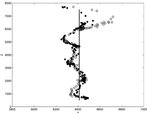
Typical closed-loop results for lowering the probe in particularly when the probe is raised from the soil,

the air are illustrated in Fig. 13. Here, it is clear that have previously led to probe repair costs of over

the SDP–PIP approach yields more accurate control £8000 on each occasion. In this regard, the present

than the linear PIP algorithm, particularly in the authors have recently developed a semi-automatic

initial positioning of the arm. In general, SDP–PIP system, whereby the operator only moves a joystick

control appears to offer smoother, more accurate either forwards or backwards in order to raise or

movement of the excavator tool and hence potentially lower the probe [24,26]. For brevity, the necessary

allows for faster response times. Note that the slew kinematic equations and rule-based algorithms for

is fixed once the probe starts to be lowered, and determining the appropriate tool-tip trajectory are

hence Fig. 13 shows only the {X, Z} coordinates, while omitted here. However, in both instances, a similar

Yremains constant during probe operations. approach to that of the laboratory excavator is

On-site implementation experiments for lowering followed (see reference [24] for details).

the probe into soil using the linear PIP controller are very promising, as reported in reference [26]. Here, 6.1 SDP models for the vibrolance

the error between the measured tool-tip trajectory and the horizontal setpoint is typically less than For this application, experimentation suggests that

a sampling rate of 0.44 s provides a good com- 10 cm for over 90 per cent of the time. To the authors’ knowledge, this level of performance is not normally promise between a fast response and a desirable

low-order model. In this case, the linear model achieved by a skilled human operator. Furthermore, the automatic system completes an entire cycle at y

k=a1yk−1+b2uk−2 again provides a reasonable

explanation of the data for a wide range of operating least as fast as a skilled human operator.

However, relatively large transient deviations from conditions. In fact, this model has been successfully

used in the design of a preliminary linear PIP control the setpoint do occasionally occur using linear PIP methods. Although these are often associated with system [26]. For non-linear design, the SDP model

of the boom takes the form of equation (4) with difficult obstructions in the soil, they provide the motivation for the present research using SDP–PIP time-invarianta

Fig. 13 Implementation experiment for the vibrolance, showing the resolved position of the end-effector, represented by the horizontal and vertical displacements (mm). Non-linear SDP–PIP control (crosses) is compared with linear PIP (circles) and the horizontal setpoint (solid)

methods. In this regard, Fig. 13 presages potential to the disturbance response. In the case of the laboratory excavator, the new approach yields improvements, and it is clear that the next step of

the research is to evaluate the on-site performance improved control of the joint angles and hence a reduced time to complete a trench. Finally, the of the new approach. Although the commercial system

used above is presently unavailable for research, the vibrolance experiments similarly suggest improved performance and robustness in comparison with the authors hope that the present paper will stimulate

further interest in this area. linear PIP methods previously developed.

ACKNOWLEDGEMENTS 7 CONCLUSIONS

The authors are grateful for the support of the Engineering and Physical Sciences Research Council This paper has developed SDP–PIP control systems

(EPSRC). Video footage of the demonstrators may for three practical demonstrators: a forced-ventilation

be downloaded from www.lancs.ac.uk/staff/taylorcj/ test chamber, a 1/5th-scale laboratory representation

nonlinear. The statistical tools and associated esti-of an intelligent excavator, and a vibrolance system

mation algorithms have been assembled as the used for ground improvement on a construction

CAPTAIN toolbox [16] within the MATLABAsoftware site. These examples represent the first practical

environment and may be downloaded from implementations of the recently proposed SDP–PIP

www.es.lancs.ac.uk/cres/captain. control methodology.

In each case, the system was modelled using the quasi-linear SDP model structure, in which the

para-REFERENCES meters are functionally dependent on other variables

in the system. This formulation is subsequently

1 Young, P. C., Behzadi, M. A., Wang, C. L., and used to design an SDP–PIP control law using linear

Chotai, A. Direct digital and adaptive control by system design strategies, such as suboptimal LQ

input–output, state variable feedback pole assign-design, in which the control gains are themselves

ment.Int. J. Control, 1987,46, 1867–1881.

state dependent. _{2 Taylor, C. J., Chotai, A., and Young, P. C.}

3 Taylor, C. J., Young, P. C., and Chotai, A. State 19 Kalman, R. E.A new approach to linear filtering and prediction problems.Trans. ASME, J. Basic Engng, space control system design based on non-minimal

1960,83, 95–108. state-variable feedback: further generalisation and

20 Bryson, A. E.andHo, Y. C.Applied optimal control, unification results. Int. J. Control, 2000, 73,

optimization, estimation and control, 1969 (Blaisdell 1329–1345.

Publishing Company, Waltham, UK). 4 Young, P. C., Lees, M., Chotai, A., Tych, W., and

21 Stables, M. A.andTaylor, C. J.Nonlinear control of Chalabi, Z. S.Modelling and PIP control of a

glass-ventilation rate using state dependent parameter house micro-climate.Control Engng Practice, 1994,

models.Biosyst. Engng, 2006,95, 7–18. 2(4), 591–604.

22 Burnham, K. J., Dunoyer, A., and Macroft, S. 5 Taylor, C. J., Leigh, P. A., Chotai, A., Young, P. C.,

Bilinear controller with PID structure. Computing Vranken, E., and Berckmans, D. Cost effective

and Control Engng J., 1999,10, 63–69. combined axial fan and throttling valve control

23 Ziemian, S. J. Bilinear proportional-integral-plus of ventilation rate. IEE Proc. Control Theory and

control.PhD Thesis, Coventry University, UK, 2002. Applic., 2004,151(5), 577–584.

24 Shaban, E. M. Nonlinear control for construction 6 Gu, J., Taylor, C. J., and Seward, D. W. The

robots using state dependent parameter models.PhD automation of bucket position for the intelligent

Thesis, Lancaster University, 2006. excavator LUCIE using the

Proportional-Integral-25 Taylor, C. J. Environmental test chamber for the Plus (PIP) control strategy.J. Computer-Aided Civil

support of learning and teaching in intelligent and Infrastruct. Engng, 2004,12, 16–27.

control.Int. J. Elect. Engng Education, 2004, 41(4), 7 Taylor, C. J., Shaban, E. M., Chotai, A.,andAko, S.

375–387. Nonlinear control system design for construction

26 Taylor, C. J., Shaban, E. M., Chotai, A.,andAko, S. robots using state dependent parameter models. In

Development of an automated verticality alignment UKACC International Conference (Control 2006),

system for a vibro-lance. In 7th Portuguese Inter-Glasgow, UK, September 2006.

national Conference on Automatic Control, Lisbon, 8 Davis, P. F. and Hooper, A. W. Improvement of

Portugal, March 2006. greenhouse heating control.IEE Proc. Control Theory

and Applic., 1991,138, 249.

9 Bradley, D. A. and Seward, D. W. The develop-ment, control and operation of an autonomous

APPENDIX robotic excavator. J. Intell. Robotic Syst., 1998, 21,

73–97.

Notation 10 Merritt, E. Hydraulic control systems, 1976 (John

Wiley, New York). _a

i{xk} output state-dependent parameters 11 Young, P. C. Stochastic, dynamic modelling and _{(i=1, 2, … , n)}

signal processing: time variable and state dependent

A(x

k,z−1) denominator polynomial parameter estimation. In Nonlinear and

non-b

b{xk} laboratory excavator boom angle stationary signal processing (Ed. W. J. Fitzgerald),

parameter 2000 (Cambridge University Press, Cambridge, UK).

b

d{xk} laboratory excavator dipper angle 12 McCabe, A. P., Young, P. C., Chotai, A., and

Taylor, C. J.Proportional-Integral-Plus (PIP) control parameter of non-linear systems.Syst. Sci., 2000,26, 25–46. b

i{xk} input state-dependent parameters 13 Hebner, A. J., Boon, C. R., and Peugh, G. H. Air _{(i=1, 2, … , m)}

patterns and turbulence in an experimental livestock _B(x

k,z−1) numerator polynomial building.J. Agric. Engng Res., 1996,64, 209–226.

c logistic growth function coefficient 14 Ha, Q., Nguyen, Q., Rye, D.,andDurrant-Whyte, H.

C

i cos(hi)

Impedance control of a hydraulic actuated robotic C

123 cos(h1+h2+h3)

excavator.J. Automn in Constr., 2000,9, 421–435.

d non-minimal state-space command

15 Budny, E., Chlosta, M., andGutkowski, W.

Load-vector independent control of a hydraulic excavator.

J. Automn in Constr., 2003,12, 245–254. f

i,k feedback coefficients at thekth 16 Taylor, C. J., Pedregal, D. J., Young, P. C., and sample (i=0, … , n−1)

Tych, W. Environmental time series analysis and _F

1,k(z−1) output feedback polynomial at the forecasting with the Captain Toolbox. Environ. _{kth sample}

Modelling and Software, 2007,22(6), 797–814.

F_i,k component of the transition matrix at 17 Young, P. C. Recursive estimation and time series

thekth sample (i=1, 2) analysis, 1984 (Springer-Verlag, Berlin).

F

k non-minimal state-space transition 18 Young, P. C.Simplified refined instrumental variable

matrix at thekth sample (SRIV) estimation and true digital control (TDC): a

g

k non-minimal state-space input vector tutorial introduction. In Proceedings of 1st European

h non-minimal state-space observation y

d,k command input at thekth sample

vector y

k control output at thekth sample k

I,k integral gain at thekth sample y2 steady-state output l

i laboratory excavator link lengths_{(i=1, 2, 3, 4)} z−i backward shift operator, z−iyk=yk−i z

k integral-of-error state variable at the l

k state variable feedback gain vector at kth sample

thekth sample p

k vector of state-dependent parameters a1 level coefficient for state-dependent

R2

T simulation fit (coefficient of parameter

determination) a

2 slope coefficient for state-dependent

S

i sin(hi) parameter

T transpose operator h logistic growth function coefficient

u

k control input at thekth sample h_i laboratory excavator joint angle (i= u

2 steady-state control input 1, 2, 3, 4)

U

k vector of exogenous variables at the H laboratory excavator bucket

kth sample _orientation

w_k vector of regression variables at the _{t samples time delay}

kth sample _{w{·} flexible logistic growth equation}

x

0 logistic growth function coefficient x_k state-dependent parameter system