Munich Personal RePEc Archive
Spillover Effects on Government Bond
Yields in Euro Zone. Does Full Financial
Integration Exist in European
Government Bond Markets?
Balli, Faruk
Massey University
May 2008
Online at
https://mpra.ub.uni-muenchen.de/10162/
Spillover Effects on Government Bond Yields in Euro Zone.
Does Full Financial Integration Exist in European Government
Bond Markets?
∗Faruk Balli
Massey University
August 25, 2008
Abstract
This paper examines the time varying nature of European government bond market integra-tion by employing multivariate GARCH models. We state that unlike other bond markets, in euro markets the default(credit) risk factor and other macroeconomic and fiscal indi-cators are not able to explain the sovereign bond yields after the beginning of monetary union. This fact might be counted as a signal for perfect financial integration. However, we also find that the global shocks affect Germany and the rest of euro bond markets in various levels, creating particular discrepancies in asset prices even we take into account the market specific factors. Different level responses of each euro market to the global shocks reveal that euro bond markets are not fully integrated with each other unlike the recent literature claimed. Besides, we explore that the global factors are effective for the volatility of yield differentials among euro government bonds.
Keywords: Financial Integration, Multivariate GARCH models. Euro Bond Markets, Spillover Effects, Asset Pricing.
JEL Classification: F15, G12,
∗Department of Economics and Finance, Massey University, Palmerston North, New Zealand. e-mail:
1
Introduction
Recently, international portfolio holders began to focus on other factors instead of standard
factors-default (credit) risk, exchange rate risk, or liquidity premium risk factors-when they
were holding euro denominated government bonds. The main reason behind the change in
investors’ decision is the recent adjustments in the formation of euro bond markets. Why does
remarkable change take place in European markets while we can not observe such a change
in the rest of the OECD bond markets? The fundamentally transformed structure of the
European bond markets has been triggered by the Maastricht treaty. In the content of the
treaty, the prospective monetary union (EMU) member aimed to satisfy certain fiscal and
macroeconomic standards to converge upon each other economically and financially by the
beginning of the currency union. To quickly summarize the criteria, the members should have
public debt levels below the Maastricht ceiling of 60% of their GDP, plus the budget deficits
of central governments should not exceed 3% of GDP. Added to these, member countries
were supposed to hold annual domestic inflation rates under 2% per annum. Expectedly, the
outcome of these policies were observed as more integrated financial markets since the mid
1990s in the euro region. Besides, both elimination of exchange rate risks and the significant
decreases in intra-euro market frictions like trading costs, brokerage commission transaction
fees, and taxes have led to a more integrated financial environment since the beginning of
monetary union.
In the first point of view, accelerated financial integration among euro bond markets has
been widely expected, since the macroeconomic and fiscal indicators have shown incredible
improvement for the “higher risk”1
euro markets, creating a potential for those members to
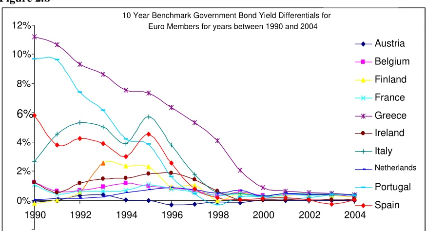
converge with “lower risk” members in terms of bond returns. Figures 2.a and 2.b present
government bond yield differentials among euro members for a time interval including the
pre and post-euro era. As illustrated in the figures, there has been a considerable decline in
government bond yield spreads since the second half of the last decade. It might be concluded
that in the wake of monetary union, bond yield convergence has been exhibited for the countries
1
experiencing higher credit(default) risk premia for their sovereign debts compared to the “low
risk” euro members.2
Although there has been such a convergence among euro area government bond yields, yield
differentials across euro bond markets have not been wiped out completely. One possibly
expect that residual spreads would definitely reflect the differences in credit standings of euro
markets, since the markets are not perfectly homogenous even after the inception of monetary
union. The Stability and Growth Pact and European fiscal frameworks appear insufficient to
guarantee that all member states have the same creditworthiness from the market point of view,
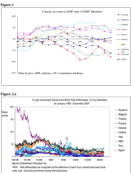
even though the Maastricht Treaty has forced the members to be in similar fiscal positions.3 In that case, euro sovereign bond yields would be counted as an important indicator of market
sensitivity to domestic fiscal exposure, since higher bond yields generally result from higher
government debt costs or higher current account deficits that require tighter market discipline
on national governments’ fiscal policies. From the portfolio holders’ point of view, it is usually
expected that those bonds tend to have higher credit risk premium. In figure 4, it is shown
that Belgium, Greece, and Italy have experienced higher debt service costs compared to other
euro members. Similarly, Portugal, Italy and Greece have been experiencing higher current
account deficits compared to the rest of the EMU members. Even though the current account
deficit/surpluses and government service debt costs are very important indicators for measuring
market sensitivity to the credit risk of government bond returns, and these measurement are
in higher levels for those markets, the sovereign bond yields do not reflect such risk premia
particularly after 1999.4
2
It is observed from historical data that Portugal, Spain, Italy, and Greece government bonds have higher default risk premia to attract cross border portfolio holders.
3
However, an important argument used by the Stability and Growth Pact opponents is that governments were not sufficiently forced to dispose of extreme government service debt and deficits. Since the beginning of monetary union, government bond yields have not effectively shown the various degrees of default (credit) risk associated with the sovereign debt issued by euro-zone central governments. It is observed that since the beginning of the common currency, there is—surprisingly—only a modest difference in the risk premia for euro-denominated central government bond yields, despite the fact that the total debt of each country differs enormously, ranging from around 30% for Ireland to over 100% for Italy, Belgium and Greece. Remaining euro countries are gathered around the Maastricht ”ceiling,” especially after 1999. Figure 3 illustrates the relationship between the average bond yield differentials for each market benchmark bond relative to the German benchmark government bond. Although we can see clear relationship between the ratings and yields, there are significant exceptions.
4
Particularly with start of the monetary union, the default risk indicators have very little
power to explain the yield spreads in the region. Theoretically, higher debt service holders’
borrowing tends to have higher risk premia compared to those holding lower debt service, but
euro government bond yields do not have such patterns robustly. A sufficient explanation
for why the default risk premium cannot be rationally observed in the euro denominated
government bond yields could be that there is a widely shared belief that even if the government
of any EMU member country threatened to not pay its debt, it would be bailed out by the
collective EMU governments. This unspoken belief makes foreign portfolio holders consider
the debt instruments of all EMU member governments as bearing the same default risk. Under
this implicit bail-out commitment, the market will treat all instruments as being of equivalent
default risk.5
1.1 The Effect of Global Shocks
Concentrating on financial asset pricing models, the recent literature finds strong evidence that
idiosyncratic properties of each market or disparate fiscal positions could straightforwardly
explain the yield spreads of government bonds between those markets. Nevertheless, after
the start of monetary union, the picture is not the same for euro bond markets. Fiscal and
other sets of indicators could barely help us explain the differentials in euro bond markets. In
other words, local factors are not as effective in explaining the yield spreads as in the periods
before the start of euro. At this time, these findings might indicate a full financial market
integration among members, since one can claim that financial asset prices no longer depend
on local risk factors. The main contribution of the paper comes out at this point. While we
control the specific market risk factors such as default risk, liquidity risk or maturity risk,
global shocks influence the government bond yield differentials among euro markets differently
and cause distortions among bond yield differentials. These findings document that for euro
bond markets, global factors play more important role in explaining the bond yield differentials
than the specific market risk does. The disappearance of default (credit) risk premium on euro
region government bond returns is associated with increasing importance of the global risk and
5
international risk factors on those bonds. In this case, we can barely talk about full market
integration given that the global shocks in the bond yields creates the deviation in the yield
differentials. We modeled the financial integration by considering both the local and global
factors and concluded that financial integration is not perfectly realized in euro bond markets.
Secondly, for the first time in the literature—up to now, the volatility of the yield spreads
were not modeled, according to our investigation of the literature—we model the volatility of
euro originated government bond yield differentials by using the Multivariate GARCH model
to control the effect of global shocks. We find that not only the yield differentials but also the
volatility of the yield differentials are affected by the global shocks, proving that full financial
integration of euro bond markets does not exist yet.
The paper is arranged as follows. In section 2, we perform a detailed literature survey,
concentrating on both the government bond markets’ integration and the effect of global shocks
through macroeconomic announcements on the markets. We discuss data issues and variable
definitions in section 3. The next section contains the empirical study explaining the yield
differentials by employing global risk factors such as macroeconomic announcements and other
international risk factors. Section 5 presents the empirical results of the Multivariate GARCH
model. The next section contains the robustness checks for the empirical models. The final
section offers concluding remarks.
2
Literature
There are a limited number of studies that have focused on measuring the integration in
gov-ernment bond markets. Besides, the literature generally used asset prices as the measurement
of the market integration. In one of the studies, Barr and Priestley (2004) tried to explain
the bond prices as being mostly related to world risk factors rather than domestic risk factors.
They argue that under full integration, exposure to purely local factors can be wiped out and
local factors will cease to have any systematic impact on expected returns. In a similar
inves-tigation, using monthly data, Codogno et al. (2003) proxy the country-specific risk factor by national debt to GDP ratios and international risk factors by U.S. markets. They find that
Austria, Italy, and Spain. Interestingly, for the latter two countries the ratio of debt to GDP
is statistically insignificant as a single variable for their studies.
Favero, Pagano and Von Thadden (2005) attempted to explain the reasons behind the bond
yield differentials in euro bond markets using various financial factors, particularly for the
period after start of monetary union. Recently, Pagano et al. (2004) have provided extensive research on the impact of the different financial and macroeconomics factors on bond yield
spreads. They focused on the importance of the international risk factors on the bond yield
differentials. Geyer, Kossmeier and Pichler (2004) estimate a state-space version model of the
time varying bond yield spreads for four EMU members. Similar to Cogodno et al. (2003), they find that global factors explain an important part of the changes in yield spreads, whereas
the local shocks have no explanatory power.
Up to this point, we have focused on literature about the steady financial integration or
limited changes with annual or monthly bases. However, financial market integration is related
to international finance, and it does make economic sense that financial market integration
changes with economic conditions. The generally accepted economic explanation is that the
level of risk aversion changes and investors require time varying compensation for accepting a
risky payoff from financial assets. Thus, more recent studies allowed integration to vary over
time and to be mostly affected by economic conditions. In this sense, financial economists
needed to study the time varying integration with more frequent databases. For example,
Aggarwal et al. (2004) and Barr and Priestley (2004) provide studies related to time-varying expected bond returns using an asset pricing model by employing daily asset prices. These
very well-known studies for the first time illustrate a time varying financial integration in
bond markets. Recently, Christiansen (2007) has used the GARCH model of Beckaert, Harvey
and Ng (2005) to assess return spillovers in European bond markets. She provides empirical
evidence that regional effects have become dominant over both own country and global effects in
EMU markets with introduction of euro but not in non-EMU countries. Although at first glance
it seems that our study is similar, we examine the full integration differently, by considering the
effect of the global shocks on asset price distortions and then employing the GARCH model. In
a parallel study, Driessen, Melenberg and Nijman (2003) find that factors relating to the term
conceivable that economic convergence required as part of EU membership has inevitably led
to high levels of bond market convergence. In a well-known study related to the integration
of European equity markets, Fratzscher (2002) has studied the volatility and return spillovers
on the European stock markets by employing a multivariate GARCH model. In addition,
he tested for cointegration—long-term relationship—in European stock markets, finding that
national stock markets mostly are integrated with each other by the beginning of the monetary
union. Also, Kim et al. (2006) examine the time varying level of integration of European government bond markets by applying co-integration tests and the GARCH model, and they
find higher levels of integration among existing European union countries than among new
members.
From a short-term perspective, some other studies have addressed market reaction to
fun-damental news released on announcement days in terms of financial asset pricing and volatility.
Such research has focused on the conditional volatility implied by ARCH/GARCH models
in-troduced by Engle (1982) and Bollerslev (1986). For example, Engle and Li (1998) examine
the degree of persistence heterogeneity associated with scheduled macroeconomic
announce-ment dates and non-announceannounce-ment dates in the treasury futures market. They present a
filtered GARCH model that takes care of cyclical patterns of time-of-the-week effects and
an-nouncement effects by decomposing returns volatility into transitory and non-transitory parts.
Regarding stock market returns, Flannery and Protopapadakis (2002) use a GARCH model
to detect the effect of macroeconomic announcements on different stock market indices. They
consider as a potential risk factor any macro announcement that either affects asset returns
or increases conditional volatility. Their results show that inflation measures, Consumer Price
Index and Producer Price Index, affect only the level of stock returns. Besides, three real
fac-tor candidates, Balance of Trade, Unemployment, and Housing Starts, affect only the return’s
conditional volatility. Similarly, Bomfim (2003) examines the effect of monetary policy
an-nouncements on the volatility of stock returns. His findings suggest that unexpected monetary
policy decisions tend to boost significantly the stock market volatility in the short run. As
expected, positive sign surprises tend to have a larger effect on volatility of the returns than
3
Data Description
The dataset for this paper includes variables, explain the government bond returns, as well
as the macroeconomic announcements published in the euro area and U.S.. To capture the
effect of the single currency on bond markets integration more effectively, we employed the
daily dataset from the starting date of monetary union, namely January 1 1999, to
Decem-ber 31 2004. The dependent variable, the 10-year euro denominated benchmark government
bond yield for each market, is acquired with daily frequency from DataStream/Thompson Inc.
DataStream uses Merrill Lynch database as a data source for the bond returns. We chose
for the start date of the dataset the beginning of the monetary union since daily prices are
regularly available through DataStream from that date. For eliminating short run
fluctua-tions in yield differentials, we utilize benchmark long-term government bonds matured in ten
years. The effect of liquidity premia on each bond market are captured accurately when we
use bid-asking spreads. Usually in the financial markets, the bid-ask spread reflects the costs
to the dealers in providing immediacy. Besides, the spreads may be affected by the level of
competition among dealers. We identify the variable as;
Liqit= Bid i
t−Askti
Aski t
.
The Bidi
t stands for the bid daily price for the given sovereign bond yieldi at timet. Askit stands for the daily asking price for the same bond in the financial markets. The spread
measures how liquid is the sovereign bond market. Apparently, the higher the spread, the less
liquid the market is. The bid-asking spread of the bonds is employed from MTS S.P.A. 6 ,
the first wholesale electronic market for government bonds. MTS is a quote-driven market in
which market-makers quote continuously two-way prices during the entire trading session for
agreed securities with a maximum bid-ask spread that depends on the characteristics of the
security.7
Another financial factor that might influence the domestic sovereign bond yields is
the maturity variable. The maturity variable is calculated by modifying the duration of the
6
Even though the dataset starts from 1999, for some of the markets, MTS does not contain bid and asking price data before 2001, the rest of the missing data is obtained from the Bloomberg Cooperation.
7
10 year government bond i. The data is taken from DataStream/Thompson Inc. To capture the effect of international risk factors on benchmark bond yield differentials in the euro zone,
we have employed various variables. Some studies on emerging markets government bonds,
including Folkerts-Landau et al. (1997) and Erbet al. (2000) documented the possible effect of the yield on U.S. government bonds or the slope of U.S. yield curve on the emerging market
bond returns. For the euro zone government markets, Blanco (2001) employed U.S. corporate
bond yields8
as a proxy for the international risk factor to explain the yield differentials among
euro government bonds. Dungey et al. (2000) conducted an empirical study to demonstrate that for euro bond markets there is also strong evidence that yield differentials are affected
by the presence of the common international factors. In this paper, considering this recent
literature, we employ two different international risk factor variables to explain the volatility
of the yield differentials. These variables are the differences between fixed interest rates on
U.S. swaps and U.S. government bond yields, and the spread between the yields on U.S. 10
year AAA rated corporate bonds and government bonds. These datasets are also gathered
from DataStream/Thomson Inc.
So far, we have defined domestic market risk factors that are previously effective to explain
the government bond yields. To assess the financial integration among the government bond
markets, we definitely need the common shock factors. In particular, we use macroeconomic
and monetary policy announcements to proxy common shocks on benchmark bond yields. The
announcements were released monthly in U.S., Germany, and the euro area during the period
of January 1999 to December 2004. We consider various macroeconomic announcements9 that
are reported to be the most influential announcements both in the academic literature and in
the press. To explain the source of the announcements briefly, in the Bureau of Statistics
PPI and CPI, retail sales and industrial production indexes are published monthly, while
the Federal Reserves FOMC meetings are scheduled eight times a year, and ECB announces
economic indicators with monthly frequency. By considering the time differences between U.S.
and euro markets, we modify the date of the announcements according to market openings in
8
Corporate bond spreads are calculated by subtracting the corporate bond index from the benchmark gov-ernment bond yield.
9
euro markets10 .
The response of bond prices to macroeconomic announcements is evaluated by utilizing the
following identity;
Kti = S i t−µit
σi t
,
where Si
t is the percentage change in the economic indicator,σti is the standard deviation of the indicator distribution and the µi
t is the mean of the distribution. Dividing differences relative to announcements to the standard deviation allows one to interpret in a consistent
manner the estimated coefficients.
4
Model
4.1 Basic Yield Differentials Model
The econometric evidence of the baseline model will explore the importance and magnitude of
common shocks on government bond yield differentials among euro members. These factors
will not only consider the macroeconomic statements observed in U.S., Germany, and the euro
area markets, but also compare the interactions between the risk factors in global markets with
the euro area risk-free bond yield spreads.
Using the daily data for the period 1999–2004, we model benchmark government bond yield
differentials in the euro zone as11 ;
∆Stig =α+ρ1∗(Liqti−Liqgt)+τ1∗(M atit−M atgt)+ v
X
h=1
̟eu
i |Kh,teu|+ y
X
j=1
̟G i |K
g j,t|+
z
X
m=1
̟us
i |Km,tus |+ε1t . (1)
10
When the announcements are released in U.S., the Euro markets are generally closed. Therefore, we utilize the effect of announcements in euro markets one business day after they were released.
11
The dependent variable is the change in government bond yield differential for benchmark
bondi over the Germany benchmark bond. Unlike the recent literature, we use the daily change in bond yield differentials as a dependent variable instead of employing yield differentials itself
as a left hand side variable and the lag of yield spreads as an independent variable, since yield
differential variables are not all stationary.12
Control variables for the local risk factors are
measured by the liquidity variableLiqi
t, the bid-asking price spread for benchmark government bond issued in countryi, and maturity variableM ati
t, the residual maturity of the particular bond. The variablesKg,KeuandKu are the German, the euro area, and U.S. announcements
respectively.13
Table 1 encloses the coefficients of macroeconomic announcements published in U.S. &
Germany presented in equation (1). The coefficients of U.S. macroeconomic announcements
are statistically significant for all regressions. Besides, macroeconomic announcements released
in Germany have positive and statistically significant effects for some bond markets in the euro
area. Table 1 contains essential results evaluating the financial integration level in the euro
region. The significant coefficients are showing that full financial integration among euro bond
markets has not existed yet, despite what some literature has claimed.
However, the reliability of the macroeconomic announcements might be questioned since
they are released in monthly frequency and might have limited effect on daily bond yield
differentials. Therefore, we alternatively employed two international risk factor variables that
obtain full set information instead of the announcements. International risk factor variables
used in the empirical model are either the spread between U.S. swap rates and U.S. 10 year
government bond yields or the difference between the U.S. S&P’s AAA corporate bond yield
index and U.S. 10-year government bond yield. The former one is issued to capture the effect of
the exchange rate risk in U.S. dollar, and the latter one contained corporate market risk
(non-diversified) in U.S. markets14
. The estimations of the regressions15
are presented in table 2.
12
Appendix Table 1 provides the stationary test results of the dependent variables. ADF test results docu-mented that not for all yield differential variables are stationary.
13
Similar stationary test has been performed for the control variables as well. We performed that the control variables are stationary.
14
Since the government bond yield is the risk free return rate and the AAA corporate bond yield index contains the market risk excluding the specific factors. The difference surrogates for the U.S. market risk factor.
15
The estimated model is,
∆Stig =η+ρ2(Liqti−Liqgt) +τ2(M atit−M atgt) +θ2(Rcor−Rsus) +ε2t , (2)
where the (Rcor −Rsus) refers to the difference between the AAA corporate bond index and
the benchmark 10 year government bond yield.16
The coefficients of the international risk
factors are significant for almost all benchmark bond yield differentials, although sign of the
coefficients are not always the same. Intuitively, having a significant coefficient indicates that
international risk factors cause divergences in yield differentials. In table 3, even when we
control both announcements and international risk factors to explain the yield differentials, we
document the significance of these factors in explaining the yield spreads.
Although the yield spreads among euro government bond markets compressed to very small
percentages, they did not vanish completely. However, they cannot be explained precisely by
the default risk factor. By employing international factors and macroeconomic announcements,
we find that euro zone government bond markets have not achieved full financial integration.
The coefficients of international risk factors and U.S. macroeconomic announcements are
sig-nificant in the first and second regression, expressed in both table 1 and 2 even when we
control for the macroeconomic announcements in Germany and other euro markets. These
results are indicating that full financial integration among the euro markets has not taken
place completely.
4.2 Multivariate GARCH Model
In Tables 1–3, we demonstrate that macroeconomic announcement effects and international
risk factors have statistically significant effects on euro benchmark government bond yield
differentials even after controlling for local market risk factors. In this part of the paper,
we measure the integration among euro bond markets by using generalized autoregressive
conditional heteroskedasticity, also known as the GARCH. This model allows us to observe
the time varying integration by considering the simultaneous effect of U.S. bond markets on
market risk has significant and positive coefficient. 16
each euro bond market return. Financial integration theories explain that the effect of global
shocks will not be statistically different from zero for different bond market returns when full
financial integration among the markets exists. By employing a multivariate GARCH model,
we observe the effect of the global shocks via U.S. bond markets on the bond yield differentials
among euro markets simultaneously. Accordingly, we will be able to reveal the time-varying
nature of euro bond market integration.
For investigating the various levels of euro market reactions to global shocks (U.S. bond
yield curve), euro markets daily bond yield differentials are modeled by considering the effect
of pair-wise yield differential equations. To obtain the spillover effect, we need to estimate
a multivariate GARCH model for euro market i, Germany and U.S. government bond yields simultaneously.
The estimated model is;
∆Stig
∆Siu t ∆Stug
=
aigt
aiu t
augt
+
T1Liqtig
T2Liqtiu
T3Liqugt
+
η1M atigt
η2M atiut
η3M atugt
+
ψtig
ψiu t
ψtug
3.a 3.b 3.c , (3) where
ψtig
ψiu t
ψugt
=
φiu φug 1
1 βug βig
ωiu 1 ωig
εiut
εugt
εigt
.
In the equations (3.a)– (3.c), the predictable model has a ∆St, the change in yield
differ-entials, includes a constant, and liquidity and maturity variables. Liqtmn is the differential of
the defined liquidity variable for market m relative to n. Similarly, M atmn
t is the differential of the defined maturity variable for market m relative to n. The unpredictable part in the model consists of innovations to change in yield differentials from the spillover effects. Say, in
equation (3.a), the unpredictable part is in the form of;
ψig =εig
t +φiu∗εiut +φug∗ε ug
εigt is the unpredictable term of equation (3.a), where,φiu∗εiu
t +φug ∗ε ug
t is the spillover term in the unpredictable part. The error termεiut andε
ug
t are the error terms of equation (3.b) and (3.c) respectively. Given that we solved the equations simultaneously with GARCH model,
we will able to plug those error terms to the equation (3.a) to get the spillover effects, namely
φiu∗εiu
t +φug∗ε ug
t , from equation (3.b) and (3.c) respectively. Similarly, volatility of bond yield differentials is modeled as;
σt2=
σtig2
σiu2
t
σugt 2
=
aigt
aiu t
augt
+
λigσig2
t−1
λiuσiu2
t−1
λugσug2
t−1
+
ωiεig2
t−1
ωgεiu2
t−1
ωuεug2
t−1
+
δiu δug 0
0 θug θig
µiu 0 µig
εiu2
t
εugt 2
εigt 2
4.a 4.b 4.c , (5)
where theσ2
t is the variance matrix of the error terms in equation (3). 17
The innovations in
equation (3),εt, are assumed to be normally distributed conditional on the past information set
that is—εt/Ωt−1— distributed as N(0, σt). σtdenotes the time varying variance, implies that
variance of the change in yield differentials in euro bond markets is determined by its own past
variance, own squared shock and by the contemporaneous squared external innovations, namely
spillover effects. In these equations we model the volatility of yield differentials among euro
government bonds by considering spillover effects of pair-wise yield differentials of each euro
bond return over U.S. benchmark bond return. The spillover coefficients 18
for the volatility
of yield differential regressions areδiu,δgu,θig,θug,µiu and µig. To make it clear, say for the
equation (4.a), the spillover effect extracting from equation (4.b) and (4.c) is in the amount of
δiu∗εiu2
t +δig∗εiu
2
t .
The theoretical framework of GARCH model in this paper is based up on the maximization
procedure of Berndt, Hall, Hall and Hausman (1974) (hereafter BHHH). The parameters are
estimated by maximizing a multivariate log likelihood function. In the multivariate case, the
part of log likelihood function becomes
17
The stationary conditions for the ARCH and GARCH model are tested. In the appendix section at Table 2 an 3, we document the stationary test results for ARCH and GARCH estimations.
18
L(θ) =−(T
2)ln(2π)− 1 2
T
X
t=1
(ln|σt|+ε
′
t σ− 1 t εt),
whereθis the parameter vector to be estimated or to be maximized, T is the number of
ob-servations andσtis the time varying conditional variance-covariance matrix. Simplex algorithm
is used to get initial values for the maximization problem. To obtain the parameter estimates,
numerical maximization is employed through the algorithm developed by BHHH(1974).
5
Empirical Results
The main contribution of this paper is to examine financial integration of euro region
gov-ernment bond markets through spillover effects. The multivariate GARCH model applied in
this analysis allows us to investigate a time-varying correlation structure for the government
bond yield differentials of each euro market bond yield relative to Germany benchmark bond
yields. Maximum likelihood estimations of the multivariate GARCH model for both euro and
non-euro bond markets are reported in Tables 4 and 5 respectively. The very first two columns
of both tables contain the coefficients of the spillover effects belonging to equation 3.a and
3.b. These columns show the spillover effect extracted from yield differentials of marketi gov-ernment bond yield over U.S. benchmark govgov-ernment bond, i.eφiu, and yield differentials for
Germany bond over US benchmark bond, i.eφgu. The results illustrate that yield differentials
of each euro government bond relative to US benchmark bonds, i.e φiu, have significant and
positive coefficients, pointing out that they have statistically significant effect on determining
the yield differentials in euro zone bond markets.
In terms of volatility, the effects of spillovers from the global factors on volatility of yield
differentials is observed clearly. The last two columns of Tables 4 and 5 represent the spillover
effect from equation (4). The coefficientsδiuandδug are measuring the spillover effects of yield
spreads of euro government bond yield for market i over US benchmark bond and German benchmark bond over US benchmark bond respectively. In these tables while performing the
GARCH model, the coefficient δiu is significant and positive for almost all euro government
affected by the yield differentials of the euro market benchmark bond over U.S. benchmark
bond. The coefficientδgu, is statistically insignificant and in terms of magnitude, infinitesimal
proving that the yield differentials between Germany and U.S. have negligible effect on the
volatility of yield differentials among euro members’ benchmark bonds. Intuitively, for the
volatility of the yield differentials, spillover parameters are basically decomposition of yield
differentials between any euro market and U.S., i.e. δiu, and Germany and U.S., i.e δug,
respectively.19
6
Robustness Checks
6.1 Germany and US market integration
Economists may claim that since the Germany bond market is fully integrated with the rest
of the OECD markets, it is expected that Germany benchmark bonds are absolutely hedged
with world markets, and the effect of U.S.-Germany bond yield differentials on the GARCH
model would be negligible—statistically not different from zero. However these expectations
could not be fulfilled with the empirical studies. The model below measures the integration of
the Germany bond market with the world bond markets.
The model is
∆Rgt =αt+βt∆Rtus , (6)
whereαis a time-varying intercept and the time-dependentβis the coefficient of integration
of the Germany bond with U.S. benchmark bond. As we explained above, for fully hedged
and integrated markets,β will converge with 1 and the intercept term will converge with zero.
Figure 5 plotsβ for the equation above. For the daily dataset between the period of 1999 and
2004, we observe that the coefficient β is far behind the level of one. This result illustrates
that U.S. and Germany benchmark bonds are not fully integrated, which is coinciding with our
findings. Besides, for non-euro countries, the spillover effect of yield differentials of German
benchmark government bonds over U.S. benchmark bonds can be observed evidently. Some
19
The coefficientsµiuandµiuare not presented in the tables. The coefficients are infinitesimal and statistically
factors, like high volumes of cross border financial asset trading with U.S. or currency exchange
risk, made some non-euro markets more integrated with U.S. bond markets than Germany.
Table 5 contains the coefficients of yield differentials from equations (3.a) and (4.a) for
non-euro countries. Spillover coefficients for Germany and U.S. yield differentials, i.e φug & δug,
are positive and significant while spillover effects from bond yield differential ofi over U.S. are not significant.
6.2 Variance Ratios
Another important method for comparing the effect of the spillover effects on each euro
mar-ket is the measurement of the volatility ratios. We can roughly define volatility ratio as a
test of measuring how much volatility of yield differentials among euro markets is explained
by spillover effects from yield differentials of euro market i government bond over the U.S. government bond, or spillover effects of yield differentials of the Germany government bond
relative to U.S. government bond.
Variance ratios are defined as ;
φiu2 εiu2
t
σtig2 , (7)
φug2 εugt 2
σtig2 . (8)
These ratios simply measure the goodness of the fit of the model. Basically, they give us
an induction about how significant the spillover effects are for the yield differential regressions.
In Figure 6.a—6.m, the ratios are illustrated for the entire period. It is observed that yield
differentials of each euro benchmark bond over U.S. benchmark bond explain yield
differen-tials among euro markets more accurately than a comparison of the yield differendifferen-tials of the
Germany benchmark bond over U.S. benchmark bond. These results denote that there are
significant variations in the bond yields among euro bond markets. Added to these, they are
and U.S., namely Eq(7), typically not by the volatility of Germany and U.S. yield differentials,
namely Eq(8). The effect of the latter one is relatively smaller.
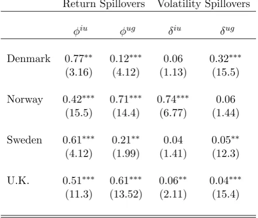
For non-euro European markets, Denmark, Sweden, and UK, the spillover effects of bond
yield differentials of euro member i over U.S. bond are relatively small compared to yield differentials of euro memberi over the Germany benchmark bond. However, the effect of the Germany benchmark bond yield differential relative to U.S. is not strong enough to explain
the fluctuations of Norway government bond yields, compared to bond yield differentials of
Norway benchmark bond relative to Germany government bonds. Since Norway government
bond market is closely correlated with German bonds recently, the Norway bond market might
has similar pattern just like with other euro markets.
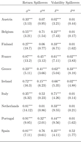
6.3 Weekly Data Estimations of Spillover Effects
For the framework of our analysis, we employed daily dataset. But there exist problems with
the international daily bond price dataset. We note that euro area shocks generally affect U.S.
returns on the same calendar day, whereas U.S. originated shocks affect European markets
only on the following day due to the differences in asset trading times. Therefore, we need
to re-perform same multivariate GARCH models by employing weekly dataset. The results
presented in Table 6 contains GARCH model estimations with weekly basis data, not basically
different from previous results. Government bond yield differentials among euro benchmark
bonds are mostly affected from the pairwise yield differentials of each benchmark bond over
U.S. benchmark bonds. The coefficients φiu
t and δtiu are positive and statistically significant whereas φgut andδgut are not.
7
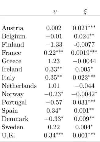
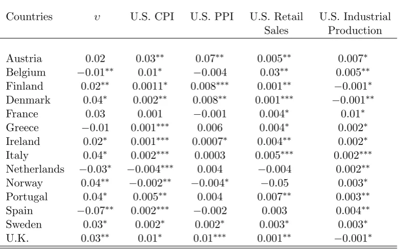
The Effects of Global Risk Factors on Spillover Effects
At this moment we relaxed the assumption that parameters of the spillover effects in
equa-tion (4.a) are fixed and we modeled the parameters as;
δtiu=ν+ξ∗Xt . (9)
sections. Tables 7 and 8 represent the effects of common news and international risk factors
on the spillover coefficients. The coefficient of ξ is positive and significant for explaining the
parameterδiu
t . Economically speaking, macroeconomic announcements, global shocks and the international risk factors have undeniably affected the spillover effects coefficients in
equa-tion(4). We can certainly conclude that the distortion of euro bond markets integration exists
due to the macroeconomic announcements released in the global markets.
8
Foreign Portfolio Decisions of Euro Area Domestic Investors:
An Alternative Explanation to Spillover Effects
Our empirical analysis indicates that even for each euro bond market, the effect of global shocks
is different. In the variance ratio analysis, it is illustrated that for pairwise yields among euro
region bond markets the differentials of benchmark bonds over U.S. benchmark bonds have
more explanatory power than euro market bond yield differentials over Germany benchmark
bonds. Euro markets have generally performed as expected, except for Greece and Ireland.
For those bond markets, the effect of yield differentials relative to Germany benchmark bonds
is significant for both return and volatility regressions. Besides, by the variance ratio analysis
, we demonstrate that the yield differentials for those benchmark bonds over Germany bonds
explain more yield differentials across the euro region as compared to the yield differentials for
those market bonds over U.S. benchmark bonds.
An alternative explanation for why Ireland and Greece lean towards the outside of the euro
markets might be that these countries’ “euro bond bias” levels20
are relatively lower compared
to other euro members. Figure 7 shows the volume of foreign bond holding portfolios of euro
countries all over the world. Investors in Ireland and Greece hold more bond portfolios from
other OECD markets instead of euro markets, whereas the rest of euro members’ “euro bias”
levels range from 60% to 80%, which are much higher than Greece or Ireland.
20
9
Concluding Remarks
The fundamentally changed structure of the European bond markets has been triggered by the
Maastricht treaty. The fiscal position of the euro members have strengthened, and previously
fiscally vulnerable members such as Greece, Portugal and Italy have experienced incredible
convergence to other euro members in terms of government bond yields. After the inception
of the euro, this convergence performance has carried on, government bond yield differentials
among these markets have decreased to very low levels. Macroeconomic indicators were not
helpful to explain the differentials at this time.
We find that after controlling the market specific factors the common news through
macroe-conomic announcements and international risk factors are important factors to explain the yield
differentials among euro benchmark government bonds. The integration of euro bond markets
is enhanced when local factors diminish their importance on yield differentials among the
mem-bers. We also find that the default risk no longer can explain the bond yield differentials in the
euro area, since high default risk premium markets might outlay lower rates of bond yields.
According to these findings, one can possibly expect that full financial integration has taken
place in euro area. However, it would not be totally true to conclude like that. Even though
default risk factors are eliminated in those markets, there are other factors that might explain
the bond yield spreads. The global risk factors-through common news-cause distortions in the
asset pricing of the government bond markets across euro bonds.
After the start of monetary union, various responses of the markets to global shocks
be-come the most important factor to explain the yield differentials in euro area bond markets.
Ultimately, we conclude that full financial integration has not existed yet in the euro bond
markets, since the global factors are still effective on the benchmark bonds in different levels.
Besides, we model the volatility of yield differentials with a time varying integration process
and find that changes in U.S. bond yield curve have a significant impact on the volatility of
benchmark bond yield differentials in the euro area. The volatility of the euro area yield
differ-entials is mostly explained by the various level responses of euro area markets to the changes in
U.S. government bond yields. We find that almost all members have experienced fluctuations
in the bond yields and these fluctuations are not homogenous across the members, creating
euro area, it is again undeniably seen that full financial integration is not achieved for these
References
Aggarwal, R., Lucey B. and Muckley C. (2004). “Dynamics of equity market integration in Europe. Evidence of changes over time and with events.” The Institute for International Integration Studies, Discussion Paper Series:019.
Barr, D.G. and Priestley R. (2004). “Expected returns, risk and the integration of interna-tional bond markets,”Journal of International Money and Finance, 23, 71–97.
Beckaert, G., Harvey C. R. and Ng A. (2005). “Market integration and contagion,” Journal of Business, 78, 39–69.
Berndt, E. R., Hall, B. H., Hall, R. E. and Hausman J. A. (1974). “Estimation and inference in nonlinear structural models,” Annals of Economics and Social Measurement, 3, 653-66.
Blanco, R. (2001). “The Euro-area government securities markets: recent developments and implications for market functioning,” Banco de Espaa, Servicio de Estudios, Working Paper 0120.
Bollerslev, T. (1986). “Generalized autoregressive conditional heteroskedasticity,” Journal of Econometrics, 31(5), 307–27.
Bomfim, A. N. (2003). “Pre-announcement effects, news effects, and volatility: Monetary pol-icy and the stock market,”Journal of Banking and Finance, 27, 133–151.
Christiansen, C. (2007). “ Volatility-spillover effects in European bond markets,” European Financial Management, 13, 923–948.
Codogno, L., Favero C. and Missale A. (2003). “EMU and government bond spreads,” Eco-nomic Policy, vol.18, 503–532.
Dickey, D. and Fuller W.A. (1979). “Distributions of the estimators for autoregressive time series with a unit root,”Journal of the American Statistical Association, 74, 427–431. Dungey, M., Martin V.L. and Pagan A.P. (2000). “A multivariate latent factor decomposition
of international bond yield spreads,”Journal of Applied Econometrics, 15, 697–715. Driessen, J., Melenberg, B. and Nijman T. (2003). “Common factors in international bond
re-turns,” Tilburg University, Center for Economic Research Discussion Paper.
Engle, R. F. (1982). “Autoregressive conditional heteroscedasticity with estimates of the vari-ance of United Kingdom inflation,” Econometrica, 50, 987-1006.
Engle, R. F. and Kroner K.F. (1995). “Multivariate simultaneous generalized ARCH,” Econo-metric Theory, 11, 122–150.
Erb C.B., Harvey C.R., Viscanta, T.E. (2004) “Understanding emerging market bonds,” Emerg-ing Markets Quarterly,4, 7–23.
Favero, C.A., Pagano M., and Von Thadden, E.-L. (2005). Valuation, liquidity and risk in gov-ernment bond markets, IGIER Working Paper no:281.
Flannery, M.J. and Protopapadakis A.A. (2002). “Macroeconomic factors do influence aggre-gate stock returns,”Review of Financial Studies,15, 751-782.
Folkerts-Landau, D., Mathieson D.J., Schinasi G.(1997) “International capital markets devel-opments, prospects, and key policy issues. IMF Staff Working Paper November 1997.
Fratzscher, M. (2002). “Financial market integration in Europe: on the effects of EMU on stock markets,”International Journal of Finance and Economics,7(3), 165–193.
Geyer, A., Kossmeier. S., Pinchler, S. (2004) “ Measuring systematic risk in EMU government yield spreads,” Review of Finance 8(2), 171–197.
Kamin, S.B. and von Kleist K. (1999). “The evolution and determinants of emerging market credit spreads in the 1990s,” Board of Governors of the Federal Reserve System, Inter-national Finance Discussion Paper No:653, November.
Kim, S. J., Moshirian F., and Wu E. (2006). “Evolution of international stock and bond mar-ket integration: Influence of the European monetary union,” Journal of Banking and Finance,30(5), 1507–1534.
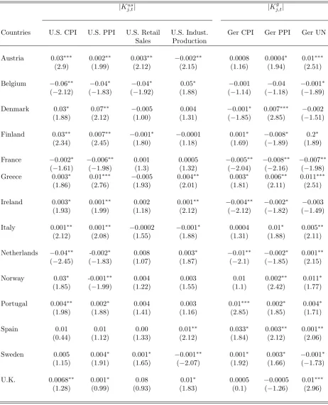
Table 1: Effect of Macroeconomic Announcements on Government Bond Yield Differentials in European Bond Markets
|Kus
j,t| |K
g j,t|
Countries U.S. CPI U.S. PPI U.S. Retail U.S. Indust. Ger CPI Ger PPI Ger UN
Sales Production
Austria 0.03∗∗∗ 0.002∗∗ 0.003∗∗ −0.002∗∗ 0.0008 0.0004∗ 0.01∗∗∗
(2.9) (1.99) (2.12) (2.15) (1.16) (1.94) (2.51)
Belgium −0.06∗∗ −0.04∗ −0.04∗ 0.05∗ −0.001 −0.04 −0.001∗ (−2.12) (−1.83) (−1.92) (1.88) (−1.14) (−1.18) (−1.89)
Denmark 0.03∗ 0.07∗∗ −0.005 0.004 −0.001∗ 0.007∗∗∗ −0.002
(1.88) (2.12) (1.00) (1.31) (−1.85) (2.85) (−1.51)
Finland 0.03∗∗ 0.007∗∗ −0.001∗ −0.0001 0.001∗ −0.008∗ 0.2∗
(2.34) (2.45) (1.80) (1.18) (1.69) (−1.89) (1.89)
France −0.002∗ −0.006∗∗ 0.001 0.0005 −0.005∗∗ −0.008∗∗ −0.007∗∗
(−1.61) (−1.98) (1.3) (1.32) (−2.04) (−2.16) (−1.98)
Greece 0.003∗ 0.01∗∗∗ −0.005 0.004∗∗ 0.003∗ 0.006∗∗ 0.011∗∗∗
(1.86) (2.76) (1.93) (2.01) (1.81) (2.11) (2.51)
Ireland 0.003∗ 0.001∗∗ 0.002 0.001∗∗ −0.004∗∗ −0.002∗ −0.003
(1.93) (1.99) (1.18) (2.12) (−2.12) (−1.82) (−1.49)
Italy 0.001∗∗ 0.001∗∗ −0.0002 −0.001∗ 0.0004 0.01∗ 0.005∗∗
(2.12) (2.08) (1.55) (1.88) (1.31) (1.88) (2.11)
Netherlands −0.04∗∗ -0.002∗ 0.008 0.003∗ −0.01∗∗ −0.002∗ 0.001∗∗
(−2.45) (−1.83) (1.07) (1.87) (−2.1) (−1.85) (2.15)
Norway 0.03∗ -0.001∗∗ 0.004 0.003 0.01 0.002∗∗ 0.011∗
(1.85) (−1.99) (1.22) (1.55) (1.1) (2.42) (1.77)
Portugal 0.004∗∗ 0.002∗ 0.004 0.003 0.01∗∗∗ 0.002∗ 0.004∗
(1.98) (1.88) (1.41) (1.16) (2.85) (1.85) (1.71)
Spain 0.01 0.01 0.00 0.01∗∗ 0.033∗ 0.003∗∗ 0.001∗∗
(0.44) (1.12) (1.33) (2.12) (1.84) (2.12) (2.06)
Sweden 0.005 0.004∗ 0.001∗ −0.001∗∗ 0.001∗ 0.003∗ −0.001∗
(1.15) (1.91) (1.65) (−2.07) (1.92) (1.66) (−1.73)
U.K. 0.0068∗∗ 0.001∗ 0.08 0.01∗ 0.0005 −0.0005 0.01∗∗∗
(1.28) (0.99) (0.93) (1.83) (0.1) (−1.26) (2.96)
Notes: Estimation method: OLS. White Heteroscedastic errors are corrected. T-statistics are in parenthesis denoting∗∗∗1%, ∗∗5%, and ∗10% significance. The estimated model is
∆Stig =α1+ρ1(Liqti−Liqtg) +τ1(M atit−M atgt) +̟eu v
X
j=1
|Ki,teu|+̟G y
X
j=1
|Kj,tg |+̟us z
X
m=1
|Km,tus |+ε1t.
∆Stig is the change in yield differentials for 10 year government bonds for country i over Germany. Liqi
t is bid-asking price spread for of 10 year government bonds countryi. M atit is modified duration of Government bonds for country i. The coefficients Keu
i,t, K g
j,t, and Km,tus are the macroeconomic announcements released in euro Area, Germany and United States respectively. Only a few of the announcement variables are illustrated. U.S. CPI, U.S. PPI U.S. Retail Sales, U.S. Industrial Production are the Consumer Price Index, Producer Price Index, Retail Sales, Industrial Production indicators released in U.S.. Similarly, Ger CPI Ger PPI, Ger UN, are the Consumer Price Index, Producer Price Index, Unemployment indicators
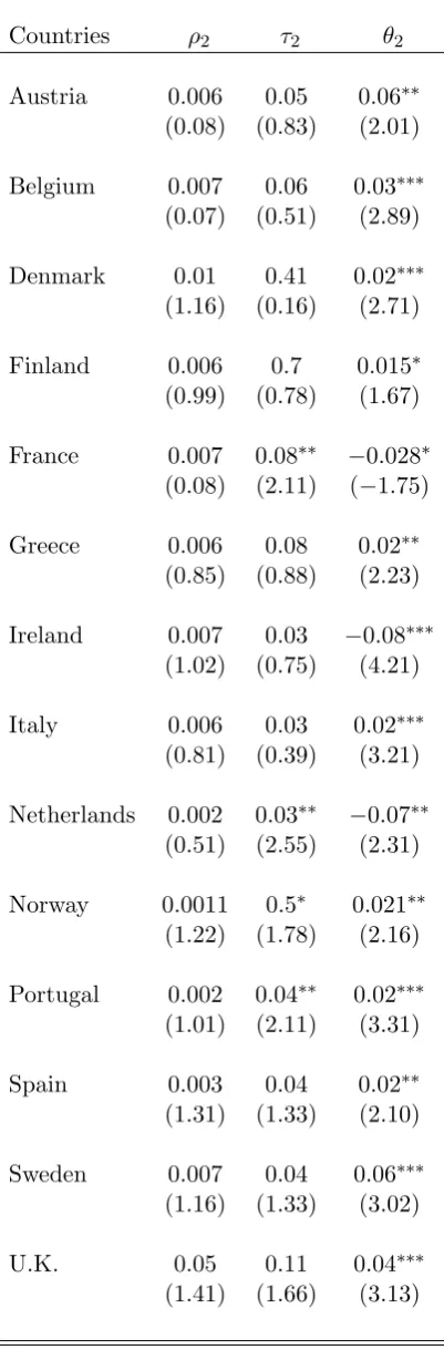
Table 2: Effect of International Risk Factors on Government Bond Yield Differen-tials in European Bond Markets
Countries ρ2 τ2 θ2
Austria 0.006 0.05 0.06∗∗
(0.08) (0.83) (2.01)
Belgium 0.007 0.06 0.03∗∗∗
(0.07) (0.51) (2.89)
Denmark 0.01 0.41 0.02∗∗∗
(1.16) (0.16) (2.71)
Finland 0.006 0.7 0.015∗
(0.99) (0.78) (1.67)
France 0.007 0.08∗∗ −0.028∗
(0.08) (2.11) (−1.75)
Greece 0.006 0.08 0.02∗∗
(0.85) (0.88) (2.23)
Ireland 0.007 0.03 −0.08∗∗∗
(1.02) (0.75) (4.21)
Italy 0.006 0.03 0.02∗∗∗
(0.81) (0.39) (3.21)
Netherlands 0.002 0.03∗∗ −0.07∗∗
(0.51) (2.55) (2.31)
Norway 0.0011 0.5∗ 0.021∗∗
(1.22) (1.78) (2.16)
Portugal 0.002 0.04∗∗ 0.02∗∗∗
(1.01) (2.11) (3.31)
Spain 0.003 0.04 0.02∗∗
(1.31) (1.33) (2.10)
Sweden 0.007 0.04 0.06∗∗∗
(1.16) (1.33) (3.02)
U.K. 0.05 0.11 0.04∗∗∗
(1.41) (1.66) (3.13)
Notes: Estimation method is OLS. T-statistics are in parenthesis. White Heteroscedastic standard errors are corrected.
The estimated model is
∆Stig =α2+ρ2(Liqti−Liqtg) +τ2(M atit−M atgt) +θ(Rcor−Rus) +ε2t.
∆Stig is the change in yield differentials for 10 year government bonds for country i over Germany. Liqi
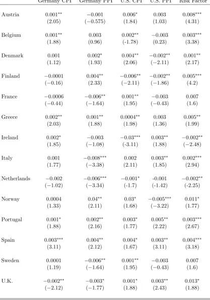
Table 3: Government Bond Yield Differentials in European Bond Markets
Germany CPI Germany PPI U.S. CPI U.S. PPI Risk Factor
Austria 0.001∗∗ −0.001 0.006∗ 0.003 0.008∗∗∗
(2.05) (−0.575) (1.84) (1.03) (4.31)
Belgium 0.001∗∗ 0.003 0.002∗∗ −0.003 0.003∗∗∗
(1.88) (0.96) (-1.78) (0.23) (3.38)
Denmark 0.001 0.002∗ 0.004∗∗ −0.002∗∗ 0.001∗∗
(1.12) (1.93) (2.06) (−2.11) (2.17)
Finland −0.0001 0.004∗∗ −0.006∗∗ −0.002∗∗ 0.005∗∗∗
(−0.16) (2.33) (−2.11) (−1.86) (4.2)
France −0.0006 −0.006∗∗ 0.001∗∗ −0.003 0.007
(−0.44) (−1.64) (1.95) (−0.43) (1.6)
Greece 0.002∗∗ 0.001∗∗ 0.0004∗∗ 0.003 0.005∗∗
(2.03) (1.88) (1.98) (1.36) (1.99)
Ireland 0.002∗ −0.003 −0.03∗∗∗ 0.003∗∗ −0.002∗∗
(1.85) (−1.08) (-3.11) (1.88) (−2.48)
Italy 0.001 −0.008∗∗∗ 0.002 0.003∗∗ 0.002∗∗∗
(1.77) (−3.38) (2.11) (1.85) (2.94)
Netherlands −0.002 −0.006∗∗∗ −0.001∗ -0.001 −0.002∗∗
(−1.02) (−3.34) (-1.7) (-1.42) (-2.25)
Norway 0.0004 0.04∗∗ 0.03∗ −0.005∗∗∗ 0.011∗
(1.33) (2.11) (1.68) (−3.22) (1.77)
Portugal 0.001∗ 0.002∗∗ 0.003∗ 0.005∗∗ 0.003∗∗∗
(1.88) (2.16) (1.77) (2.22) (2.67)
Spain 0.003∗∗∗ 0.004∗∗ 0.004∗ 0.003∗∗ 0.004∗∗∗
(3.11) (2.12) (1.67) (3.11) (3.18)
Sweden 0.0001 −0.006∗∗ 0.001∗∗ −0.003 0.007
(1.19) (−1.64) (1.95) (−0.43) (1.6)
U.K. −0.002∗∗ −0.003∗ 0.001∗ 0.003∗∗ 0.013∗
(−2.12) (−1.77) (1.88) (2.43) (1.88)
Notes: Estimation method is OLS. White Heteroskedastic errors are corrected. T-statistics are in parenthesis denoting ∗∗∗1%,∗∗5%, and∗10% significance. The estimated model:
∆Stig =α3+ρ3(Liqti−Liqtg) +τ3(M atit−M atgt) +φ3(Rcor−Rus) +̟,G y
X
j=1
|Kj,tg |+̟, us
z
X
m=1 |Kus
m,t|+ε3t.
∆Stig is the change in yield differentials for 10 year government bonds for country i over Germany. Liqi
t is the bid-asking spread of traded bonds. M atit is the residual maturity. (Rcor −Rus), international risk factor, is the spread between 10-year AAA corporate Bond yield index and the yield on 10-year US government bonds. U.S. CPI, U.S. PPI U.S. Retail Sales, U.S. Industrial Production are the Consumer Price Index, Producer Price Index, Retail Sales, Industrial Production indicators released in U.S.. Similarly, Ger CPI Ger PPI, are the
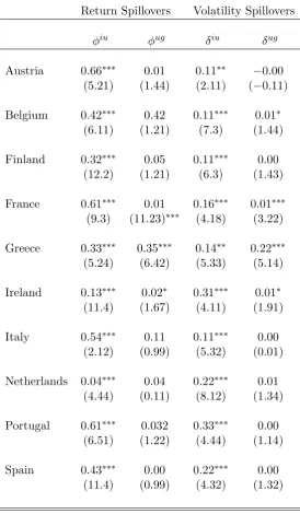
Table 4: Multivariate GARCH Model for Euro Government Bond Returns
Return Spillovers Volatility Spillovers
φiu φug δiu δug
Austria 0.66∗∗∗ 0.01 0.11∗∗ −0.00
(5.21) (1.44) (2.11) (−0.11)
Belgium 0.42∗∗∗ 0.42 0.11∗∗∗ 0.01∗
(6.11) (1.21) (7.3) (1.44)
Finland 0.32∗∗∗ 0.05 0.11∗∗∗ 0.00
(12.2) (1.21) (6.3) (1.43)
France 0.61∗∗∗ 0.01 0.16∗∗∗ 0.01∗∗∗
(9.3) (11.23)∗∗∗ (4.18) (3.22)
Greece 0.33∗∗∗ 0.35∗∗∗ 0.14∗∗ 0.22∗∗∗
(5.24) (6.42) (5.33) (5.14)
Ireland 0.13∗∗∗ 0.02∗ 0.31∗∗∗ 0.01∗
(11.4) (1.67) (4.11) (1.91)
Italy 0.54∗∗∗ 0.11 0.11∗∗∗ 0.00
(2.12) (0.99) (5.32) (0.01)
Netherlands 0.04∗∗∗ 0.04 0.22∗∗∗ 0.01
(4.44) (0.11) (8.12) (1.34)
Portugal 0.61∗∗∗ 0.032 0.33∗∗∗ 0.00
(6.51) (1.22) (4.44) (1.14)
Spain 0.43∗∗∗ 0.00 0.22∗∗∗ 0.00
(11.4) (0.99) (4.32) (1.32)
Notes: T-statistics are in parenthesis denoting ∗∗∗1%, ∗∗5%, and ∗10% significance. The
esti-mated model is
∆Stig =aig+T1(Liqit−Liqgt) +η1(M atit−M atgt) +φiuεiut +φugεugt +εigt .
σigt 2 =αig +λigσtig−21+ωigε ig2
t−1+δ
iuεiu2
t +δugε ug2
t .
Table 5: Multivariate GARCH Model for Non-Euro Government Bond Returns
Return Spillovers Volatility Spillovers
φiu φug δiu δug
Denmark 0.77∗∗ 0.12∗∗∗ 0.06 0.32∗∗∗
(3.16) (4.12) (1.13) (15.5)
Norway 0.42∗∗∗ 0.71∗∗∗ 0.74∗∗∗ 0.06
(15.5) (14.4) (6.77) (1.44)
Sweden 0.61∗∗∗ 0.21∗∗ 0.04 0.05∗∗
(4.12) (1.99) (1.41) (12.3)
U.K. 0.51∗∗∗ 0.61∗∗∗ 0.06∗∗ 0.04∗∗∗
(11.3) (13.52) (2.11) (15.4)
Notes: T-statistics are in parenthesis denoting ∗∗∗1%, ∗∗5%, and ∗10% significance. The
esti-mated model is
∆Stig =aig+T1(Liqit−Liqtg) +η1(M atit−M atgt) +φiuεiut +φugεugt +εigt .
σtig2 =αig+λigσtig−21+ω igεig2
t−1+δ iuεiu2
t +δugε ug2
t .
Table 6: Multivariate GARCH Model for Euro Government Bond Returns with Weekly Data
Return Spillovers Volatility Spillovers
φiu φug δiu δug
Austria 0.33∗∗∗ 0.07 0.02∗∗∗ 0.01
(3.13) (0.95) (3.21) (0.44)
Belgium 0.55∗∗∗ 0.71 0.22∗∗∗ 0.01
(3.21) (1.54) (7.43) (0.17)
Finland 0.27∗∗∗ 0.06 0.33∗∗∗ 0.01
(18.7) (0.77) (6.71) (1.62)
France 0.87∗∗∗ 0.45∗∗ 0.61∗∗∗ 0.02∗∗∗
(13.2) (3.12) (7.11) (3.83)
Greece 0.23∗∗∗ 0.41∗∗∗ 0.62∗∗ 0.33∗∗∗
(5.11) (3.66) (5.04) (8.18)
Ireland 0.72∗∗∗ 0.15∗∗∗ 0.66∗∗ 0.02∗∗∗
(16.3) (6.23) (5.35) (4.88)
Italy 0.35∗∗∗ 0.52 0.71∗∗∗ 0.01
(6.32) (0.23) (4.26) (0.14)
Netherlands 0.81∗∗∗ 0.01 0.33∗∗∗ 0.01
(14.12) (0.86) (9.55) (0.21)
Portugal 0.91∗∗∗ 0.32∗∗ 0.44∗∗∗ 0.01
(9.85) (2.01) (9.56) (1.62)
Spain 0.81∗∗∗ 0.76 0.35∗∗∗ 0.52
(7.11) (0.61) (4.11) (1.77)
Notes: T-statistics are in parenthesis denoting ∗∗∗1%, ∗∗5%, and ∗10% significance. The
esti-mated model is
∆Stig =aig+T1(Liqit−Liqtg) +η1(M atit−M atgt) +φiuεiut +φugεugt +εigt .
σtig2 =αig+λigσtig−21+ω igεig2
t−1+δ iuεiu2
t +δugε ug2
t .
Table 7: The Effect of International Risk Factors on Spillover Coefficients
υ ξ
Austria 0.002 0.021∗∗∗
Belgium −0.01 0.024∗∗
Finland −1.33 -0.0077 France 0.22∗∗∗ 0.0019∗∗∗
Greece 1.23 −0.0044 Ireland 0.33∗∗ 0.005∗
Italy 0.35∗∗ 0.023∗∗∗
Netherlands 1.01 −0.044 Norway −0.23∗ −0.0042∗
Portugal −0.57 0.031∗∗∗
Spain 0.34∗ 0.001∗∗
Denmark −0.33∗ 0.009∗∗
Sweden 0.22 0.004∗
U.K. 0.34∗∗∗ 0.001∗∗∗
Notes:The estimated model is
σtig2 =aig+λigσ ig2
t−1+ω
igεig2
t−1+δ
iuεiu2
t +δugε ug2
t . (4.a)
We relaxed the assumption of the parameters for spillover are fixed:
δtiu=υ+ξXt.
∗∗∗1%, ∗∗5%, and ∗10% are denoting significance. Xt is the variable for measuring the