Design of optimal control systems and industrial applications

Design of optimal control systems and industrial

applications.

FOTAKIS, Ioannis E.

Available from Sheffield Hallam University Research Archive (SHURA) at:

http://shura.shu.ac.uk/19659/

This document is the author deposited version. You are advised to consult the

publisher's version if you wish to cite from it.

Published version

FOTAKIS, Ioannis E. (1981). Design of optimal control systems and industrial

applications. Doctoral, Sheffield Hallam University (United Kingdom)..

Copyright and re-use policy

See

http://shura.shu.ac.uk/information.html

POND iE E I , SHEPH^LD S I 1WB _ J hl°lf

Sheffield City Polytechnic Library

ProQuest Number: 10694540

All rights reserved

INFORMATION TO ALL USERS

The quality of this reproduction is dependent upon the quality of the copy submitted.

In the unlikely event that the author did not send a com plete manuscript and there are missing pages, these will be noted. Also, if material had to be removed,

a note will indicate the deletion.

uest

ProQuest 10694540

Published by ProQuest LLC(2017). Copyright of the Dissertation is held by the Author.

All rights reserved.

This work is protected against unauthorized copying under Title 17, United States C ode Microform Edition © ProQuest LLC.

ProQuest LLC.

789 East Eisenhower Parkway P.O. Box 1346

Design of Optimal Control Systems and Industrial Applications

Ioannis Emmanuel Fotakis

Coll a b o r a t i n g Establishment :

Swinden Laboratories

British Steel C o r p oration

A thesis presented for the CNAA degree of Doctor of Philosophy.

Department of Electrical and Electronic

Engineering

Sheffield City Polytechnic

qx

C

Design of Optimal Control Systems and Industrial Applications

I E Fotakis

Abstract

This thesis describes work on the selection of the optimal control criterion weighting matrices, based on multivariable root loci and

Summary of Contributions

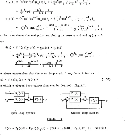
1. The first solution of the finite time LQP optimal control problem for discrete time systems in the z-domain including a closed loop form output feedback solution for the regulator and tracking problems. (jL, 2^

2. The combination of a Kalman filter with the MacFarlane-Kouvaritakis design technique

QQ.

3. The design of a control scheme for a Sendzimir steel mill to be implemented by the British Steel Corporation in their Shepcote Lane mills [4, 5^] .

Papers published or to be published

1. J Fotakis and M J Grimble: "Solution of Finite Time Optimal Control Problems for Discrete Time Systems", presented on Conference on Systems Engineering, Coventry 1980.

2. M J Grimble and J Fotakis: "Solution of Finite Time LQP Optimal Control Problems for Discrete-Time Systems", submitted for publication to Trans ASME.

3. J Fotakis, M J Grimble and B Kouvaritakis: "A Comparison of

Characteristic Locus and Optimal Designs for Dynamic Ship Positioning Systems", to be published IEEE Transactions on Automatic Control, 1981.

4. M J Grimble and J Fotakis: "Strip Shape Control Systems Design for Sendzimir Mills", invited presentation at IEE Decision and Control Conference, Albuquerque, 1980.

5. M J Grimble and J Fotakis: "The Design of Strip Shape Control

ACKNOWLEDGEMENTS

A PhD thesis, being the result of three years of research work,

naturally involves the co-operation, consultation and discussion with

many people. I should like to thank everybody concerned.

I would like to express my appreciation to my supervisor, Dr M J

Grimble, for his guidance and encouragement all through the period of

this research work. Also to the staff of the Department of Electrical

and Electronic Engineering, particularly to Dr W A Barraclough.

I am grateful to all the friends whose discussions cleared up points

and brought new ideas; I would especially like to thankDr B Kouvaritekis

of Oxford University.

Thanks are also due to our industrial collaborators at British

Steel Corporation, Swinden Laboratories, Rotherham, specifically Dr M Foster

and Mr K Dutton of the Systems Division. Finally, I should like to thank

CONTENTS

Abstract

Summary of Contributions

Acknowledgements

CHAPTER 1

Introduction to Optimal Control Problems

CHAPTER 2 .

Optimal Control Systems with Cross-Product Weighting; Weighting Matrices Selection

CHAPTER 3

Finite Time Optimal Control for Discrete-Time Systems

CHAPTER 4

The Design of Strip Shape Control Systems for a Sendzimir Mill

CHAPTER 5

A Comparison of Characteristic Locus and Optimal Control Designs in a Dynamic Ship Positioning Application

CHAPTER 6

Concluding Remarks

References

CHAPTER 1

An Introduction to Optimal Control Problems and Methods

1•1 Introduction

There have been continuous advances in theoretical control

engineering over the last twenty years, particularly in the field of

Linear Systems. The work of Kalman is notable in this respect. During

the last decade, frequency domain techniques for multivariable systems

have been developed by Rosenbrock, Mayne and MacFarlane and their co­

workers [18,19,20]. The implementation of new control techniques has

led to systems with tighter specifications and better performance. As

control engineers take into account the overall needs of the process

to be controlled, changes in the priorities of the objectives to be

fulfilled lead to the development of appropriate control schemes.

A trend in the design of industrial systems is to consider energy

losses in the process and the trade off between system performance and

minimization of energy losses. To quantify this improvement, a cost

criterion has to be defined. The controller which minimizes this cost

function may be found using Optimal Control theory. The use of optimal

control theory comes very naturally in the area of aero-space vehicle

trajectory control and the design of aircraft control systems. In the

following, optimal control will also be shown to provide a framework

for the design of certain industrial systems.

As with the main body of control engineering results, the main

particular considering quadratic terms in the cost function. The main

advantages of Linear Quadratic Optimal Control feedback systems stem

from (i)the ease of obtaining the solution to a particular problem

4

once the weighting matrices of the performance criterion are defined;

(ii)the guaranteed asymptotic stability of the closed loop system and

(iii)its direct and easy applicability to systems with many inputs and

outputs. The main disadvantage of optimal control when applied to

industrial problems where criteria like step response, overshoot, rise

time, etc. , are of prime importance, is that there are few results

relating those specifications to the weighting matrices of the

performance criterion. In recent years a number of authors have

presented papers trying to overcome this difficulty and have described

methods of designing such optimal systems.

In the present thesis some contribution is made towards the

problem of weighting matrices selection as described in chapter two.

The solution to the finite discrete time optimal control problem is

described in chapter three. The following chapter deals with the i

design of the shape control scheme for a Sendzimir cold rolling mill.

Chapter five gives a detailed comparison between an optimal controller

(obtained using the design methods of chapter two) and one designed

with multivariable frequency domain techniques. An overview of the

research effort follows in the concluding chapter.

-1.2 Complex Frequency Domain Approach to Systems Analysis and Design

The s-domain approach to control systems analysis and design was

developed by Wiener during the Second World War years. His famous

dissertation on these methods was often refered to as the 'ye^ ow

peril'. This stemmed from the yellow cover of the then classified

report [l]. In this fundamental treatise on the subject he introduced

several ideas which have been incorporated in later work. These may be

classified as follows:

(i) Formulation of the filtering and control problems using optimal

cost functions and solutions of these problems using s-domain or

Parseval theorem approaches.

(ii) Use of the spectral factorisation in the optimal control

solution.

(iii) The requirement that the optimal control or filtering solution

has to be realised by causal components and the means to achieve this

condition.

Wiener's work was classified during the war years but soon after

was further developed by other researcher's such as Newton et al [2 ].

Although the s-domain approach created some interest it was never

applied in multichannel filtering or multivariable control problems

and the number of real applications were very few. The later work by

Kalman [3,4] in the time domain (since 1960) found immediate

application in the aerospace industry and in many other fields. In

some ways the problem formulation and solution were very similar, the

only differences lying in the form that the solution was achieved. The

state feedback solution to the control problem was found to be

particularly appropriate. Similarly the recursive solution to the

-estimation problem enabled filtering algorithms to be implemented

easily on digital computers. The calculation of either the optimal

control feedback gain matrix or the Kalman filter gain matrix reduced

to the solution of a matrix Riccati equation. This difference between

the Wiener and Kalman approaches is crucial. The solution of most of

the linear quadratic optimal control and estimation problems was

reduced to the solution of only one sort of matrix equation which

enabled computer solutions to be obtained for general system

descriptions. The Wiener approach however cannot be systematised in

this way. Each problem and system description must be treated

individually and the solution procedure cannot be implemented via a

standard algorithm.

The s-domain approach taken here does not overcome this later

problem^ however the class of problems considered is wider than that

considered up to now in the literature. Although not treated in this

thesis there is a method recently developed which may offer a solution

to the problem of achieving standard algorithms. Peterka [6] and

Kucera [5] have developed a polynomial equation approach to systems

theory which goes some way towards providing standard solutions.

Kucera has proposed algorithms for most of the calculations involved

in the polynomial matrix solutions. However there are no applications

in this area and computer packages are not yet available nor likely to

be, within the next two or three years.

Other authors have made contributions in the area of s-domain

analysis and design. Yula et al[7] in a relatively recent paper on

Wiener-Hopf methods introduced one new important component into the

problem solution. They recognised that the solution to optimal control

-problems do not necessarily lead to stable closed loop configurations.

They were considering the output feedback situation where a cascade

controller is used. For example if a plant is non-minimum phase and a

straight-forward minimum variance controller is designed [8] the

closed loop system can be unstable. To avoid this situation the

problem can be refoimulated and in this case the minimum variance

controller by Peterka [6] is obtained which leads to a stable closed

loop system. In the former case the optimal controller tries to cancel

the right half plane zeros of the plant and thus creates unstable and

uncontrollable poles. Hidden unstable modes always result in closed

loop unstable systems and must therefore be avoided.

To circumvent the above difficulties Yula et al proposed that the

control problem specification should be altered to include stability

as well as optimality. This extra restriction is manifested in the

control solution by additional constraint equations which must be

satisfied. These authors were considering infinite time optimal

control problems and they did not develop algorithms which could be

implemented on computers.

Few authors have considered the solution of finite time optimal

control problems. There are two main reasons, first that finite time

optimal controllers and filters are more complicated than their

infinite time counterparts and second that most filtering and

estimation problems fall more naturally into the infinite time problem

structure. However Grimble [9] and Fotakis and Grimble [lo] have

developed a frequency domain approach to the solution of these

problems. In chapter three the z-domain solution of the deterministic

finite time optimal control problem is described. This procedure has

the disadvantages mentioned above; that is, it is difficult to derive

-a gener-al -algorithm for the multiv-ari-able c-ase -and finite time

problems are not so often found in industrial situations. However, one

important role for this approach has been found where these

limitations are not so important. This is in the design of optimal

controllers for self tuning applications, where the disturbances are

of a deterministic rather than a stochastic nature. For example these

disturbances may be represented by sudden steps into the plant

(instead of white noise). The applications of these controllers in

self tuning systems is not considered in the present thesis but the

theoretical ground work is presented which will enable such

controllers to be designed. It is of interest to note that self tuning

controllers based upon optimal control criteria using k-step ahead

cost functions are directly related to the deterministic controllers

proposed here (for the infinite time situation). The solution of the

finite time optimal control problem has not been obtained previously

in the z-domain by other authors.

-1.3 Frequency Domain Multivariable Design

Many authors have considered the design of systems in the

frequency domain, notahly Bode, Nyquist and Evans for single input

single output systems and Rosenbrock and MacFarlane for multivariable

systems. The design of optimal systems in the frequency domain has

attracted little attention. Grimble [ll] and Fotakis [12] have

recently developed a method of specifying the Q, R and G weighting

matrices of the performance criterion using frequency domain criteria.

The hope is that gain and phase margin type of information may be

specified and from this the performance criterion can be developed.

One of the difficulties of this approach is that the criteria so

specified do not completely define the Q and R matrices. The positive

aspect of this is that this freedom in the selection of the matrix

elements may be employed fruitfully by the designer. In the same time

this causes difficulties in the attempt to program the method as a

standard algorithm for the design of systems. However it is hoped that

an interactive computer aided design facility (CAD) may be used to

overcome this problem. The designer would use the constraints imposed

by the frequency domain requirements to partly specify the weighting

matrices and then, as at present, use his engineering judgement to fix

the remaining elements of the matrices.

Although other authors (eg MacFarlane [13]) have considered the

frequency domain properties of optimal systems, few have considered

the design of such systems in the frequency domain. The work described

here must be extended to incorporate other design criteria, but the

simple examples given, show that the performance indices used have

produced systems with reasonable response characteristics.

-1.4 Review of the basic Optimal Control results

A brief review of the optimal control problem approaches both in

s-domain and in state space formulation follows. Considering the

linear time invariant plant described by the equations:

x( t)=Ax(t)+Bu(t) (1.1)

j(t)=Cx(t) (1.2)

and the criterion:

J(u)=<y(T), ^ y ( T )>+J(<y( t) f Qy( t)>£+<u( t), Ru(t)>|dt (1-3)

the problem of determining the control u(t) for 0<t<T which minimises

the criterion J(u) is known as the deterministic linear optimal

control regulator problem [15]- Because of the equation 1.2 the

criterion j(u) may be rewritten as:

j(u)=<

As has been proven [14 ,15] the solution to this problem can be obtained

from the matrix Riccati equation:

u(t)=-R“1BtP(t)x(t) (1 .4)

- H t)=CtQC-P( t)BR“1 B ^ C t )+P( t)A+AtP( t) (1.5)

with terminal condition P(t)=C^P^C (1 * 6)

This solution is given in a block diagram representation in figure 1.

A second way of obtaining the control u(t) is through augmentation of

the state space equations, by considering the cosystem (or adjoint) of

system (A,B,C). The optimal trajectories are given by the equations

[16]:

x(t) A BR’V x(t)

f i t) CtQC -At x (t)*/ \ (1

this solution is depicted in figure 1b and is equivalent to the x(T), CtP <1Cx(T)>+/(<x(t), CtQCx(t)>+<u( t), Ru(t)>)dt

I “ SrK, " *“ ~ ~

-matrices C^QC and R should be both positive definite. It is

interesting that the nature of the problem leads to a state feedback

closed loop system and this is asymptoticaly stable if and only if the

pair (A,B) is stabilizable [37].

Next consider the criterion

j(u)=<e(T), P1e(T)>+/(<e(t), Qe(t)>+<u(t), Ru(t)>)dt (1.9)

1 ^Jo ' c.r

with e( t)=y(t)-r(t) (1 .10)

where r(t) is the desired output and e(t) is the error between actual

and desired output. This problem is known as the deterministic linear

optimal control servomechanism. The solution may be obtained either

using the Riccati equation or by considering the cosystem equations:

(

.

)

x (t)=C^QCx(t)-A^x (t)+C^Qr(t)

This solution is shown in figure 2a. The Riccati equation solution is

u(t)=-R~1 B*?(t)x(t)+R“1 Btg(t)

-?(t)=CtQC-P(t)BR"1P(t)A+AtP(t) (1.12)

g(t)=(AtP(t)BR“1B^)g(t)+CtQr(t)

with P(T)=CtP1C and g t T ^ - C 1^ r(T)

and this is depicted in figure 2b. It is clear that both problems

have the same solution structure and the same closed loop properties.

The frequency domain solution is reviewed next: first the system

operator W relating input and output is defined through the well known

convolution integral of the impulse response matrix w(t) with the

system input:

y( t) = (¥u) ( t ) = t - t ) u ( t )dx (1-15)

*“ 0

the criterion J(u) (of equation 1.9) can be expressed as follows by

-J(u)=<e, Qe> +<u, RuX = <(r-Wu), Q(r-Wu)> + <u, Ru> _{— “ “ H r ~ ~ - rtr} (1 . 1 4 )

From this relationship a gradient function g(u) may he defined and

the necessary condition' for optimality is that g(u)=0 £ 17D•

Transforming this into the s-domain and using spectral factorisation

[73] the solution is found as [17]:

u(s)=[Y(s)]“1 i[Yt(-s)]"1W t(-s)Qr(s)]+

=F(s)r(s) (1*15)

and Yt(-s)Y(s)=Wt(-s)Q¥(s)+R

and a feedback closed loop controller can be obtained as:

K(s)=F(s)[l-W(s)F(s)]"1 (1-16)

and this form of solution is shown in figure 2c.

-1

1

CHAPTER 2

2.1 Introduction

In dealing with the design of optimal controllers for industrial

applications there has been two main criticisms. The first concerns

the selection of the performance criterion weighting matrices and the

second is the apparent need for phase advance [21, 22],This is only a

problem when an observer is required for the implementation of the

state feedback controllers. The phase advance in LQP systems follows

because the determinant of the return difference matrix is greater than

unity for all frequencies. [23,24] This implies that for a single

input system the phase margin [25] is greater than 60°. To be able to

have a smaller phase margin the locus of detF(s) must pass within the

unit circle, and this can be achieved for an optimal system if a cross

product weighting term, between the state and the control, is intro­

duced. In this chapter such a problem is defined, its properties are

studied and a design procedure is outlined.

To help with the selection of the weighting matrices, use is made

of recent results [33,34] on the asymptotic root loci properties of

optimal systems. The use of root locus to design optimal systems

originated by Chang [30] and was extended by Tyler and Tuteur

[31]-The relationship between the Q and R matrices and conventional design

characteristics has been investigated but there are not any results

for the multivariable case [ 32 ]. Chen and Shen [ 33 ], Solheim [ 34 ]

produced algorithms for this purpose but their methods have the

weakness of considering only the eigenvalues of the system. Harvey

and Stein [ 35 ] considered the state regulator problem when the system

is controllable observable and minimum phase. In this work the output

regulator is considered and the plant is assumed to be stabilisable

and detectable only.

-The initial development of the design technique presented in this

Chapter was described in Grimble [22], [36] . The author contributed

to the theoretical analysis and was responsible for the computer

implementation and the applications of the technique to the industrial

problems.

-2.2 Optimal Control Problem

We consider the following linear constant plant, controllable

and observable represented by the state space equations:

x(t) = Ax(t) + Bu(t) (2.1)

y(t) = Cx(t) (2.2)

with A,B,C the plant matrices and define as performance criterion

*00

J(u) = \ <£(t), Qe(t)>£ + <u(t), Ru(t)>£

• J0 r m

+ 2<y(t), Gu(t)>E + 2<y(t), Mr(t)>£ (2.3)

r d

where the weighting matrices Q and R are positive definite and the

error e(t) is defined as the difference between the plant output

from the desired output r(t):

£(t) = r(t) - 'y(t) (2.4)

To obtain a unique solution for the above optimal servomechanism

problem the two cross product weighting matrices G, M have to be

constrained. These constraints are obtained by .rearranging equation

2.3 ti remove the cross product terms:

<u, Ru>e + 2<y, Gu>E =

m r

= <u + R_1GTy, R(u + R_1GTy)>E - <R"1GTe, GTe>E

m m

- 2<y, G R ^ G 1^ + <R“1GTr, GTr>E (2.5)

r m

T

by choosing M = G R " ^ both the cross-product matrices depend upon G

and if we set:

Q; = Q - GR_1GT (2.6)

UjCt) = u(t) + R-1GTi (t) (2.7)

the performance criterion may be rewritten as: r co

J(u) = I <e(t), Q xe_(t)>E + <ui(t), Rux'(t)>E dt (2.8)

r m

-where the last term in the identity 2.5 is omitted from the criterion

since it is constant for any defined r(t) and does not affect the

minimisation of J(u). The original plant is equivalent to the

following:

x(t) = A xx(t) + Bui(t) (2.9)

y(t) = Cx(t) (2.10)

where Aj = A - BR“1G^C (2.11)

It is clear that a constraint for G comes from equation 2.8

where Qi a 0, that is

Q - GR"1GT > 0 (2.12)

The optimal control Uj(t) for the criterion 2.8 and plant 2.9

leads to the desired control u(t), for the original problem, through

equation 2.7. Both, the original system (A,B,C) and the system (A^,B,C)

have the same state trajectories, for the same initial conditions.

All the above results apply to the state regulator problem (by setting

the matrix C equal to the unity matrix) and to the output regulator

by setting the reference t: = 0. It is well known that the state

feedback solution for the optimal control problem is obtained by the

Riccati differential equation and for the infinite-time problem, from

the algebraic Riccati equation.

-2.3 Return difference, Optimality condition

The frequency domain solution to the above problem is obtained

as follows. Define the optimal state feedback matrix Kx:

Kx = R“1BTP x (2.13)

which leads to the control law (see also section 1.4):

UjCt) = -Kjx(t) + R - ^ (2.14)

or for the original plant

u(t) = -(Kx + R71GTC)x(t) + R-',BT£

= -10c(t) + R_1BT£ (2.15)

where

K = K2 + R_1GTC (2.16)

Now for the infinite time case the matrix P2 is the positive

semi-definite constant matrix obtained from the algebraic Riccati equation:

-PlAx - aJp2 + P1BR"1BTP1 = CTQxC ' (2.17)

We consider the matrix return difference of the examined system:

F(s) = I + K<Ks)B (2.18)

where

4>(s) = (sI-A)'1 (2.19)

and the plant transfer function is W(s) = C.<j>(s)B (2.20)

The optimal return difference equation follows after substituting

into equation 2.17, equation 2.11 and 2.13:

-P2A - ATP! + KXTGTC + CTGKx + Kx^Kx = CTQxC (2.21)

so we have

P l ^ s ) - 1 + 4>T (s)"1Px = CTQxC -

I x V c

premultiplying by B $ (-s) and post multiplying by cf>(s)B and using

2.16 leads to

WT (-s)QxW(S) + R + WT (-s)G + GTW(s) -f WT (-s)GR_1GTW(s)

= FT (-s)RF(s) (2.22)

-This equation can be rewritten by use of equation 2.6 as

WT (-s)QW(s) + R + WT (-s)G + GTW(s) = FT (-s)RF(s) (2.23)

or

WT (s)Q!W(s) + (I + WT (-s)GR"1)R(I + R“1GTW(s)) =

= FT (-s)RF(s) (2.24)

Equation 2.23 becomes identical to the one discussed by '

MacFarlane (23,2^in the case where the crossproduct term G vanishes.

The above equation applies direct to the original optimal control

problem; the equivalent transformed one is useful only for supplying

the constraints on matrix G (equation 2.12).

MacFarlane Hfj has shown for the case with no crossproduct term the

necessary condition for optimality is

|det F(ja))|* 1 V we R (2.25)

This implies that the Nyquist locus plot of det F(ju)) .lies outside

the unit circle with centre (0,0) and for a single input plant this

means that the phase margin will be greater than 60°Q25j. This is out

of the range of the usual design criteria and is a.drawback if state

feedback can't be applied because it requires a significant amount of

phase advance to be introduced by a dynamic compensator which can

cause noise problems.

By the use of the crossproduct term (matrix G) we can prove that

the above equation (2.25) need not be satisfied.

Let v(s) be an eigenvector of F(s) corresponding to the eigenvalue

p(s):

F(s) v(s) = p(s).v(s) T

premultiplying equation (22) by v (-s) and postmultiplying by v_(s) we

obtain:

-vT (-s)WT (-s) QW(s)v(s) +vT (-s)[R + WT C-s)G + GTWCs)]v (s) =

= P("s)p(s)vT (-s)RV(s)

because the term in Q.is positive semidefinite on the jtu axis o£ the

s-plane the above equation leads to the following necessary

condition for optimality:

1'

O*OP

* -T(-jco) [R 7 T(-i,)G <

(2 26)

v C-jo))Rv(jo))

T T . •

in this equation IV (-jw)G + G W(jio) is Hermitian but not positive

definite and thus only when G = 0 the above gives |p(ju))|2 £ 1 for

all a). By use of the relation: n

det F(jco) = n p-(jw) i=l

we see that the condition 2.25 does not necessarily apply when a

cross-product term exists. Similarly the criteria developed by Porter [26j

do not hold in this case. From the above we can conclude that the

necessary condition for optimality becomes

|det F(ja))| £ r^ (2.27)

where r^ is the radius of a circle which can be less than unity.

If Q and R are predetermined it may not be possible to choose G

so that the det F(joi) locus can enter the unit circle because G must -l T

also satisfy the condition of equation 2.12 Qi = Q - G R : G £ 0.

So we will assume that Q, R a G can be chosen freely to satisfy

equation 2.12 and equation 2.27 for a desired value of r^ < 1 so we

are not going to evaluate r£ using equation 2.26 which would be a

quite.difficult task.

From equation 2.23:

|det F(jcu) |2.det R =

= det [WT (-jai)QW(jto) + R + WT (-ju))G + GTW(ja3)] (2.28)

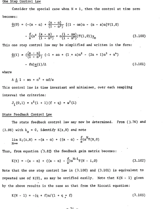
-Figure 1 depicts a plot of det F(jio) for a system with

cross-product weighting. The point of origin is the critical point for

stability so for an open loop stable plant the feedback system will

be stable if the origin is not enclosed. Hsu and Chen have shown [27]:

n

Jl (s - Yj)

det F^sj = (2.29)

n (s - X.) i=l

where y. are the closed-loop system eigenvalues and X^ are the open

loop system eigenvalues (eigenvalues of the plant matrix A ) .

The minimum distance from the origin to the plot of det F(jw) is

a measure of the degree of stability of the system. And in this method

of design this distance is specified in the beginning together with the

frequency at which det F(joj) touches the circle of radius r^. It is

found that this point is often very close to the phase margin point

which is the point the det F(j(u) plot is cut by a unit circle with

centre (1,0). This result is useful as it defines the frequency range

up to which the optimal feedback system gives an improvement in

sensitivity over the open loop system [25,28^

Rosenbrock and McMorran Q>l| have also shown that as the frequency

tends to infinity det F(jw) tends to the (1,0) since the system is

proper and it approaches that point with an angle of -90°.

-I (det F (jejJ))_m

det F (jto) plane

critical point

for stability unit circle

0.6 radius circle .

R (det F (jui)) -1

-1

Figure 1 Frequency response plot of det F (jo))

-2.4 The Design Method

With optimal control for a given plant the design reduces to the

selection of the weighting matrices Q, R, G. In all the design methods

the usual procedure is an iterative process of trial and error until

a satisfactory performance of the closed loop system is obtained. The

.same holds here for this method. In the literature some ways are

described of how to choose Q and R to achieve certain conventional

system performance characteristics like steady-state error, peak

overshoot etc. Those ideas can be applied properly modified to cal­

culate the G matrix.

The design procedure has the following steps:

1) Choose the radius r^ and frequency wm which is the minimum of

det F(jaj), o)m can be chosen very near to the desired system

bandwidth or phase margin frequency of the fastest loop in a

multiloop system.

2) Expand Q-GR_1G $ 0 to obtain a set of inequalities which must be

satisfied by the elements of Q, R and G.

3) Evaluate ~ ( | d e t F(ja))|2) = 0 and set w = (2.30)

Obtain also the equality

det[WT (-ju))Q.W(j<i3) + R + WT (-jo))G + GTW(ju)] _ 2 fo ,11

det R ' r£ 1 -1

This is the necessary condition that |det F(jw)| has minimum

rr at to ._{f m}

4) Collect all equalities and inequalities the elements of Q, R, G

must satisfy from steps 2, 3.

5) Choose Q, R, G such that the above relationships and any other

conventional criteria are satisfied.

-Example 1

We consider the following single input three output plant

originally considered by Fallside and Seraji(293 for the case with

G = 0.

-1 0 0 "1”

X = -1 0 -2 x + 0

_0 1 -1 _0_

u (2.32)

y = 1 3x

The performance criterion is j(u) =

where Q = diag(qxq2q 3) R = 1 G = (gig2g3)

The open loop transfer function matrix is

<3C, Qx> + <u, Ru> + 2<xy Gu>dt

T

W(s) = u (s)_{* o J}

T 2 + s + 2

-(s +

)

-1

(2.33)

pQ (s) = (s+1)(s2+s+2) = s3+2s2+3s+2

In general restricting Q to be diagonal matrix can result in no

feasible solution but in this case with diagonal Q there exists a solution;

we choose g^ = g3 = 0 .

A(s) = WT (-s)QW(s) + R + WT (-s)G + GTW(s) =

p (s )p ~C-T j [qi (s2- s+2) .«12 C *-1). -qs] S+S+2

-Cs+

)

-1

or A(io) =

+ 1 + —_{pQ (s)} g2 (s-1) ♦ —_{pQ (s)} (-g2 (s+l))

(o^ - aco** - 8w 2 + y , A o o --- where a = 2 - q^ - 2g2

(06 - 2(0^ +(02 +4 _{3 = 3qi - q2 + 2g2 - 1}n i (2.34)

y = 4qx + q2 + q 3 + 4 - 4g2

-for the local minimum -7— = 0

aw

(a-2)w2 + (2+28)w 6 + (12-d-28-3y)w **

v ' m m y m

+ (4y-8d)wm2 - (y+48) = 0

and |A(wm)|2 = r£2

T*

the restriction on G: Qi = Q - GR_1G 5 0 qi a 0 q2-g22 j 0

q 3 5 0 (2.35)

For w = 8 rad/sec rr = 0.7_{m t}

we have:

— ■= 0 /. 16777216(a-2) + 524288(1+8) + 4096(12-a-28-3y) + 256(y-2a)

- (y+48) = 0

16772608a + 5160928 - 12033y = 32980992

|A|2 = rf2 : 4096a + 648 - y = 13764.

since there is no other requirement any solution of 2.34 which

satisfies the inequality 2.35 is acceptable. By letting A(o) = 10^ so

the d.c. gain F(o) = 102 gives:

y = 410*+

a = 56.56

8 = -843.8

and from 2.34:

qi = 1 g2 = -27.28

q2 = 790.24

q3 = 39091

The optimal gain matrix becomes:

K = [6.634 -55.92 -128.81]

and the initial condition responses are shown in the figure 2 these

are similar to the responses that Fallside and Seraji obtained but also

-the system has a more realistic phase margin.

For the same system but for = 5.5 rad/sec r£ = 0.7 we get the

solution

qi = 2 g2 = -10

q2 = 102

q3 = 2

which gives K = [.6637 -9.884 .7214]

and the responses for this case are shown in figure 3.

An attempt was made to computerise the above design algorithm but

the effort was abandoned as the estimated programming time was far more

than was available and there was inadequate library routines to obtain

solution for the non linear system of equalities and inequalities.

-ST

AT

ES

0.6

0.2

TIME (SECS)

- 0.2

Q * diag'(l 790.24(1 24 39091} 0 -27.78 0-1T Figure .2 Initial Condition Responses

0

8

0.6

4

2

0 0

- 0 . 2 TIME (SECS)

2.5 Selection of the Performance-Criterion Weighting Matrices

Let us consider the same plant (A,B,C) as defined in equation

2.1, 2.2, with the further assumption that the system is square. This

assumption can be justified since the outputs defined through

equation 2.2 need not to coincide with the actual plant outputs; for

example, additional outputs may be defined to square up the system.

Also CB is assumed full rank; the more general case when CB is not full

rank is discussed later. The performance criterion to be minimized has

the following form: *00

J(u) = <y(t),Qy(t)>£ + y2<u(t),Ru(t)>E

•*0 m m

+ y<y(t),Gu(t)>E dt (2.36)

m

where Q, R are constant symmetric positive definite matrices and G

A T

is constant and Qi = Q - GR”1G is positive definite as shown

previously. Let us denote by S the mxm full rank square root of

Ql: = S .s and the pair (A,S) is assumed to be detectable. The

control weighting depends on the real positive scalar y. The solution

of the above problem is the same as before (equations 2.14 to 2.23)

excep.t for the inclusion of y:

u(t) = -K3c(t) (2.37)

K = (R”1/y2)(BTP 1 + yGTC) = R_1BTPx/y2 + R_1GTC/y

= Kx + R”1GTC (2.38)

-PxA - ATPx + yKxTGTC + yCTGKx + y2KxTRKx = CTQxC (2.39)

this final steady state matrix Riccati equation gives rise to the

equivalent frequency domain equation:

y2FT (-s)RF(s) = W T ( -s) Q W (s) + y2R + yWT (-s)G

+ yGTW(s) (2.40)

The expressions for calculating the weighting matrices Q and R are

obtained from the following theorem. The crossproduct matrix G is not

determined by these results but as already described it can be chosen

to shape the system time response and has to satisfy the conditions T

set above; furthermore G CB has to be symmetric or G is null 9

Theorem 2.1 Selection of Q and R

For the LQP problem defined above assume that m pairs (X^ v^ )

are specified. The optimal control weighting matrices can be selected

to provide the given asymptotic behaviour, for y-H):

Q = [(CBN)T]“1(CBN)”1 (2.41)

and

r = (NT)"1A0V 1 (2.42)

where N = {vx” , ^ 00, ... vj”} and A°° = diag{ (lAx*50)2, (1/X2°°)2 ,... (1/Xm°°)2}

As y-K) there are m infinite closed loop eigenvalues of the form

= X i 7 u (2.43)

I 09 I

where |X^ | < °° with m corresponding closed loop eigenvectors:

CO 00 . . «

x. = Bv- (2.44)

— l — i

Proof of Theorem 2.1

The proof relies on results from optimal root loci theory and the

closed loop eigenvector relationships summarised in Appendix 1. It

is shown that the return difference matrix F(s) determines the vectors

v^ through the relation

F(Xi)vi = 0 (2.45)

for each X^£ cr(A).^ Thus the frequencies {X^} are a set of closed-loop

eigenvalues and the vectors {v^} relate to the closed loop eigenvectors.

The asymptotic behaviour of the closed loop system poles, is as

follows:

As shown in Appendix 2.1 (ti-m) closed loop eigenvalues remain finite as

00

y->0. The rest of the m closed loop eigenvalues {X^ /y} approach

-infinity in m first order Butterworth patterns [38]. These

eigenvalues must necessarily be a subset of the controllable modes, since

the uncontrollable modes are invariant under feedback, that is, the

oo

asymptotically infinite modes A^ /yj£cr(A). The eigenvectors corresponding

to the (n-m) finite modes are discussed later in section 2.7, now the

eigenvectors corresponding to the m infinite modes are determined as following.

Let $(s) be expanded as a Laurent series [39] then W(s) may be written 1

W(s) = CCs"1^ + s"2A + s~3A2 + ...) B (2.46)

From the above equation 2.40 gives:

U2FT (-S)RF(S) = y2{R - ^p-[(CB)TQCB + 0(l/s)]

- — [(CB)TG - GTCB + 0(1/s)]} _]iS (2.47)

T T

Assuming that G satisfies the condition (CB) G-G CB = 0 and

denoting si = ys equation 2.47 becomes

FT (-s)RF(s) = R - - \ [ ( C B ) TQCB + 0(l/s)] - -i-0(l/s) (2.48)

S1 ^1

thus for a given finite frequency sj, as y-H) then |s|-*» and

FT (-s)RF(s)+ R - — ^2t(CB)TQCB (2.49)

From equations 2.45 and 2.49 for each finite frequency A^°°

corres-00 00

ponding vector v^ and infinite eigenvalue A^ = A^ /y:

FT (-Ai)RF(Ai)vi°° = 0 (2.50)

[ R — (CB)TQCB]v.°° = 0 (2.51)

( X f ) 2

T

As Q is symmetric positive definite it may be written Q = E E with

E full rank, this substituted in the last relation:

[((ECB)T)‘1R(ECB)‘1]ECBv.” = i — ECBv.” (2.52) (Xi

The above is an eigenvector equation, the matrix within the square

-brackets is positive definite and symmetric, therefore has positive

real eigenvalues (1/x/”)2 and orthogonal eigenvectors ECBv^00. Assume

the magnitude of these eigenvectors to be unity and define

then

- CO 00 CO- _

-N = (vj , v2 , } (2.53)

(ECBN)T (ECBN) = I (2.54)

If N is supposed to be specified then Q follows from equation 2.54:

Q = [(CBN)1]"1(CBN)"1 (2.55)

The matrix E may be chosen as E = (CBN)-1 which is full rank (m) but

is not symmetric. Then equation 2.52:

> T _ i CO 1 l 00

(N RN)N xv. = — -— N_1v.

1

a”)2 1

from which if A°° is defined as A = diag{l/(Xi)2 ,- 1/(X2)2, •••

R = (NT)"1A°°N":l

Thus the infinite modes are given by X^ = X?/y as y-H) and the

associated eigenvectors are x^ = Bv^ as shown in Appendix 1.

00

In the case where N is chosen as the identity then R = A is

r p

diagonal, Q = [(CB) ]_1 (CB)"1 and as s^^EIV^-H^/s, further more, if

CB is diagonal then Q will be diagonal also.

-2.6 Calculation of the weighting matrices, Example

As it was shown the weighting matrices Q and R depend on the

00 00

choice of the frequencies X^ and the vectors V^, but even when the

matrix G is null (absent from the performance criterion) the process

is not complete. The finite value of y must be selected and this

may lead to a modification of Q and R so that all the specification

requirements are fulfilled. The full design process is discussed' in

later sections.

The m closed-loop asymptotically infinite eigenvalues determined. 00

by the m frequencies X^ may be selected to achieve given bandwidth

requirements on the inputs. As an example, for a two-input system with

the actuator corresponding to input 1, ten times as fast as that for

00 00 00

input 2, then Xi = IOX2 . The frequency Xi may also be normalized, so

XT = -1 and x” = -o.l. The vectors v” may be chosen so that the

associated inputs are decoupled at high frequency. That is, the matrix

N may be defined to be a diagonal matrix. An alternative method of

selecting the m-pairs (xT,v?) is to consider the desired output

bandwidth and interaction. Define the asymptotic output directions

as:

00 00 00

y. = Cx. = CBv. (2.56)

— 1 — 1 —1

where i = {l,2,...,m}. Since CB was assumed full-rank

v” = CCBrV”

;

(

.

)

00

and thus the vectors may be chosen so that there is low interaction

in the outputs between the fast and slow mode terms. That is, if

M = [yj, ,y°°] then M may be defined to be a diagonal matrix.

-Example 2 Output Regulator Problem

Consider the open-loop system discussed by Moore [AO]. The system

matrices are defined as:

“ 1.25 0.75 -0.75

A = 1 -1.5 -0.75

1 -1 -1.25

B =

1 0

0 1

0 1

1 0 0

0 0 1

Let the weighting matrix G = G and note that CB = I2 . This plant is

stabilizable but not controllable. For a finite-gain non-optimal system

Moore chooses the following desired output directions:

Li

-0.9

0.32

y£

= cx

=

0.1

corresponding to desired modes A 2 = -5 and A3 = -6 , respectively. These

are taken below as the required asymptotically-infinite output directions

and modes, and the Q and R matrices are determined.

For this problem CB = I2 and v^ = y\ thence

“ 0.9 1 N =

and from (2.56)

0.32 0.1

Q = ( N Y N" = (NNT)" 0.6687 1.1184

1.1184 10.767 (2.58)

-T i °° i

R = ( N ) _1A N"1 = 0.0193 0.0238 0.0238 0.3718

Note that

T C QC

0.6687 0 1.1184

0 0 0

1.1184 0 10.767

and thus in the equivalent state regulator problem state 2 is not weighted.

The time responses for this system are shown in figures 4 to 4eand these

responses are discussed in the next section.

-2.7 Asymptotically Finite Modes

The expressions for the matrices Q and R were obtained by con­

sidering the behaviour of the m asymptotically infinite modes. The

equations which determine these modes and the associated closed-loop

eigenvectors were also obtained before. In the following the signi­

ficance of the remaining (n-m) asymptotically finite eigenvalues and

eigenvectors is discussed and the defining equations are obtained.

This set of eigenvalues contains any uncontrollable modes. The

relationship between the asymptotically finite closed loop poles (also

referred to as optimal finite zeros) and the system zeros has been

discussed by Kouvaritakis [3*f] and is summarised below.

Theorem 2.2 Asymptotically Finite Modes

The asymptotically finite closed-loop poles of a square minimum

phase system S(A,B,C) are equal to the zeros of S(A,B,C). The

asymptotically finite closed-loop poles of a square non-minimum phase

system S(A,B,C) are given by the union of the set of left-half plane

zeros of S(A,B,C) together with the set of the mirror images of the

right-half plane zeros of S(A,B,C) about the imaginary axis.

Proof: The proof given by Kouvaritakis £3*0 depends upon the augmented

system S(A*,B*,C*) defined in appendix 1. The system zeros are

defined in appendix 3.

Note that the cross-product weighting matrix does not affect the

above results (Appendix 1) even when the assumption made in section 2.5

does not hold.

It will now be shown that if the plant is assumed to be minimum

phase the asumptotically finite eigenvectors lie within the kernel of

C. Thus uncontrollable modes for example, will not be present in the

output responses which is a highly desirable practical objective. The

following theorem, developed by Kwakemaak is now required on

-the maximum achievable accuracy of regulators.

Theorem 2.3 Maximum Achievable Accuracy

Consider the stabilizable and detectable linear system 2.1, 2.2

(B and C full rank) with criterion 2.36 (Q, R > 0 and G = 0) then

lim J(u) = 0, if and only if, the transmission zeros of S(A,B,C) lie y->o

in the open left-half complex plane [41, 42]

Corollary 1 Asymptotically Finite Eigenvector Directions

The asymptotically-finite eigenvector directions {x?} for the

minimum phase plant W(s) lie within the kernel of C, that is Cx? = 0,

for j e (1,2,___,n-m}.

Proof: The output may be expressed [40] in terms of the eigenvalues

Xj (the asymptotically finite eigenvalues are assumed distinct) and

eigenvectors x_j as follows:

n m Xit

y(t) = Z Cx. (£. x J e

j=l "I 3 ~° (2.59)

rn

where p^ ... g^] = [x^ X £ ,.... x^l”1, Assume now that Cx^ ^ 0 and

since Xq is arbitrary, assume that the output contains a non-zero term

in e^*. Each output component is therefore composed of n

linearly-independent terms on C(0,«) and at least one component must include a

term in e“^'t. The cost-function weighting matrix Q > 0 and thus

lim J(u) ^ 0 =t»W(s) is not minimum phase. It follows from the y-K>

contradition that Cx^ = 0.

Corollary 2 First Order Multivariable Structure

The closed-loop transfer function matrix T(s) for the square

system S(A-BK°°, B, C) is of first-order type [43, 44j .

Proof: The closed-loop eigenvalues are assumed distinct and thus the

matrix A-BK°° has a simple diagonal structure and T(s) may be expressed

in the dyadic form:

-T

n Cx._z. B m a. T

T(s) = i=i W = 3h T i ^ T ^ (2'60)

where.the set of dual eigenvectors is denoted by {z^} and the

asymptotically finite eigenvectors (belonging to the k e m a l of C) have

been omitted in the second summation. A square multivariable system

that has the dyadic structure in 2.60 was defined by Owens [43] to be

of first-order type.

Theorem 2.4 Asymptotically Finite Eigenvector Directions

Consider the optimal control problem described in theorem 2.3 and

assume that the plant S(A,B,C) is minimum phase, and the assumptions

given in section 2.5 hold .The (n-m) asymptotically finite eigenvalues

and eigenvectors are related to the system zeros and zero directions

as follows:

(a) The (n-m) asymptotically finite eigenvalues {A°} are equal to the

(n-m) zeros of the system S(A,B,C).

(b) The asymptotically finite eigenvector x° > corresponding to the

eigenvalue A°, is identical (except possibly for magnitude) to the

state zero direction u k, corresponding to the zero X?.

o A 00 o

(c) The asymptotically finite input vector = -K x. is identical

(except possibly for magnitude) to the input zero direction a?,

corresponding to the zero A°.

Proof: Part (a) follows immediately from theorem 2.1. From

corollary 1 of previous section the asymptotically finite eigenvalue

A? and eigenvector x? satisfy

(A?I - A + BK°°)x? = 0 | A? | < oo (2.61)

3 -J J

Cx° = 0, for j e {1,2,...,n-m} (2.62)

The definitions of zeros and zero directions are given in appendix 3.

Note that the above equations are satisfied for a given limiting gain

-matrix K (as p-K)). It follows from theorem A3.2 in appendix 3 that

A? is a zero of the system S(A,B,C) and x° is the corresponding state

zero direction. Conversely, if (A?,x?) denotes a zero and state zero

direction of the system S(A,B,C) and if this zero is assumed to have

unit algebraic and geometric multiplicity [45], then the vector w? is

unique (except for magnitude). Thus, identify w? = x? and part (b) of

the theorem follows. Finally, part (c) of the theorem follows from a

similar argument, given the above assumption.

The following theorem holds for a more restrictive set of

conditions.

Theorem 2.5 (Harvey and Stein [ 35]^ 1978)

Consider the LQP optimal control problem described in section 2

with the additional assumptions that the plant is controllable and

observable and minimum-phase. Also assume that the transmission

zeros of W(s) do not belong to the spectrum of A and are distinct.

As p-K) the (n-m) finite closed-loop eigenvalues {\°} and associated

input vectors v? are defined by:

W(X°)v? = 0 |X°| < « (2.63)

and the corresponding closed-loop eigenvectors x° are given by:

x? = (A?I - A)"1Bv? (2.64)

— J 3 n — J

for j e {1;2,...,n-m}.

Proof: From equations (2.40) and (2.45) the (n-m) finite eigenvalues

satisfy (as p-K))

WT (-X°)QW(\°)v° = 0, for j e {1,2,...,n-m} (2.65)

The stable closed-loop eigenvalues must therefore satisfy (2.64).

The closed-loop eigenvector (2.65) follows directly from corollary

A2.1 and theorem A2.2 in appendix 2.

-The results of this section for minimum phase plants may be

summarised as follows. As p-K) (n-m) closed-loop eigenvalues

remain finite and approach either the transmission zeros of W(s) or

invariant zeros of S(A,B,C). The system has the desirable charac­

teristic that all uncontrollable modes (assumed less than n-m)

become unobservable. The closed-loop transfer function matrix for

the system, as p-K), has a simple dyadic structure and the system is

of first-order type. The asymptotically finite eigenvector

directions define (A,B) invariant subspaces [46,47] in the kernel

of C.

The situation described above is not the same as that discussed in

section.2.5, regarding the asymptotically-infinite modes. These modes

and the corresponding eigenvectors are determined by the weighting

matrices which are specified by the designer (via the (X^v^) pairs).

However, the asymptotically finite modes are determined by the plant

structure. The zeros and zero directions may only be varied by

changing the combinations of inputs and outputs from the plant which

may not be possible. The above results are nevertheless useful in

design since they allow the (n-m) asymptotically closed-loop

eigenvalues and eigenvectors to be calculated before the weighting

matrices are chosen.

-Example 3 Calculation of the Asymptotically Finite Modes

The finite zeros and zero directions, for the output regulator

problem may be determined using the results of Kouvaritakis and MacFarlane [48]

The invariant zeros are found by determining matrices N and M such that

NB = 0, CM = 0 and NM = I , and then computing the eigenvalues of the

matrix NAM. Thence, NAM = -0.5 and the system has the invariant zero

Si = -0.5. [49]. Notice that this zero corresponds with the position of the

uncontrollable mode. The transfer-function matrix has the form:

W(s) = _P0Cs) "(s + 0.5) (s + 2.25) 0

(s + 0.5) (s + 0.5)(s + 1.25)

Sil - A B _*i

c o_

where PQ (s) = (s + 0.5)(s + 1.25)(s + 2.25). Clearly the assumption that

the zero does not belong to the spectrum of A does not hold in this example,

The state and control zero directions can be found from the more general

theorem 2.4. These directions may be calculated as follows:

= 0

thence

X! = [0 4 0]T

£1 = [3 -4]T

The above invariant zero is also an input decoupling zero for the plant

(the number of input decoupling zeros = rank defect of the controllability

matrix = 1).

The time responses for various values of y, are shown in figures 4d T

to 4e. The initial state is assumed to be = (0 0 1) . As y tends

to zero the two outputs tends to zero almost everywhere. However, the

uncontrollable mode has a dominant influence on state 2. This clearly

indicates that the eigenvector corresponding to the uncontrollable

-mode belongs to the kernel of C. It is also evident that this eigenvector

direction does not change significantly for finite non-zero y, since the

uncontrollable mode does not dominate the outputs for such values of y. The

system responses compare'favourably with those obtained by Moore [40] 1

-X3 (output 2)

.90

4.0 3.0

2.0

1.0

.80

(output I)

co

I

o

*

$_a .00

3.0 2.0

80 a.

a a

X2

Cb) '

30 2.0

-•ca

t*

and

ou

tp

ut

ma

gn

it

ud

e*

»ta

t*

and

ou

tp

ut

ma

gn

it

ud

e*

3.0

.00

XI (output 1)

X2

X3 (output 2)

3.0

.00

3.0

2.0

Xt (output 1)

0.0 i

-Fig. 4: State and Output Responses

-2.8 Locus of the Closed Loop Poles as y Varies

An initial finite-value for y may be selected by choosing the

distance of the faraway closed-loop poles to the origin and by using

the relationship established in Appendix 4. If for example this

radius or distance is chosen as r^, then y^ becomes:

y,. = — (a2 det Q/det R)2m (2.66)

rf

where a is the coefficient of s in the zero polynomial W(s); that is,

a = det CB. In example '-'"2 det Q = 5.95, det R = 0.00661, r^ = 5.5,

m = 2 and a = 1, thence y^ = 0.996 (Figure 5).

The values of Q, R and y^ so defined, are good starting points

for a design, however, it is very likely that the value of y^ will

need modification. A suitable value for y^ may be selected from optimal

root-loci plots for the system [j3, 55]. The root-loci start at the

points for which y-*», which correspond to low feedback gains. In this

case the closed-loop poles approach either the open-loop stable poles

for the plant, or the mirror images of the open-loop unstable poles.

These results are summkrized in Appendix 2.5. The root-loci tend

towards either the plant zeros or the infinite zeros, as y-K). This

case was discussed in previous sections and corresponds to the use

of high state-feedback gains Q>0j.

It is clearly desirable to have an efficient root locus plotting

program. Such a program may be developed using the primal-dual system

discussed in Appendix 1 and a multivariable root locus plotting

package (as discussed by Kouvaritakis and Shaked [51]). However, in

the present design method the alternative approach of calculating

the eigenvalues of the closed loop system matrix Ac = A - BK is more

desirable, since eigenvectors may also be easily calculated. Efficient

algorithms are readily available for eigenvalue/eigenvector calculations.