Generating Scenario Trees for Multistage
Decision Problems
Kjetil Høyland • Stein W. Wallace
Department of Industrial Economics and Technology Management, Norwegian University of Science and Technology, N-7491 Trondheim, Norway
[email protected] • [email protected]
I
n models of decision making under uncertainty we often are faced with the problem of representing the uncertainties in a form suitable for quantitative models. If the uncertain-ties are expressed in terms of multivariate continuous distributions, or a discrete distribution with far too many outcomes, we normally face two possibilities: either creating a decision model with internal sampling, or trying to find a simple discrete approximation of the given distribution that serves as input to the model. This paper presents a method based on non-linear programming that can be used to generate a limited number of discrete outcomes that satisfy specified statistical properties. Users are free to specify any statistical proper-ties they find relevant, and the method can handle inconsistencies in the specifications. The basic idea is to minimize some measure of distance between the statistical properties of the generated outcomes and the specified properties. We illustrate the method by single- and multiple-period problems. The results are encouraging in that a limited number of generated outcomes indeed have statistical properties that are close to or equal to the specifications. We discuss how to verify that the relevant statistical properties are captured in these speci-fications, and argue that what are the relevant properties, will be problem dependent. (Scenario Generation; Asset Allocation; Nonconvex Programming)1. Introduction and Motivation
In models of decision making under uncertainty, it is essential to represent uncertainties in a form suit-able for computation. If random varisuit-ables are repre-sented by multidimensional continuous distributions, or by discrete distributions with large numbers of out-comes, computation is difficult because the models explicitly or implicitly require integration over such variables. To avoid this problem, we normally resort to either internal sampling or procedures that replace the distribution with a small set of discrete outcomes. In stochastic programming, which provides the moti-vation for this paper, internal sampling is used in models of stochastic decomposition (see, for example, Higle and Sen 1991) and importance sampling (see, for example, Infanger 1994 and the references therein).We can also resort to sampling when a continuous distribution is to be represented by a discrete approx-imation. To make sure that the distribution properties of the sample are close to those of the continuous dis-tribution, the number of outcomes has to be large. However, this may easily result in another situation where the decision model fails because of the implied integration. Therefore, there is a need for a means of generating the outcomes in a more intelligent way than by sampling, irrespective of whether that sam-pling is stratified or not.
process, discretizing the continuous probability distribution.
The standard approach for approximating a contin-uous distribution by a discrete distribution is the fol-lowing: (1) divide the outcome region into intervals, (2) select a representing point in each interval, and (3) assign a probability to each point. An example of such an approach is the “bracket mean” method. The intervals are found by dividing the outcome region into N equally probable intervals, the representative point is the mean of the corresponding interval, and the assigned probability is 1/N. Miller and Rice (1983) point out that “bracket mean” methods always under-estimate the even moments and usually underesti-mate the odd moments of the original distributions. They illustrate a method that overcomes this flaw. The procedure, which is based on Gaussian integration rules, generates anN-point distribution that matches the first 2N−1 moments of the continuous distri-bution. Smith (1993) reviews different methods of constructing discrete distributions, and proposes an efficient method for accurately computing the moments of an “output distributions” (or value lot-tery) given the moments of the input distribution. Keefer (1994) draws attention to the fact that even though the discrete distribution matches the first several moments of the continuous distribution, the approximation of the expected utility (EU) or cer-tainty equivalent (CEV) (which are the bases for the decisions) can be poor. He proposes six different three-point approximations that lead to quite accu-rate estimations of the CEVs when the risklevel and the continuous distributions are within reasonable bounds.
Some of the literature described above discusses
multiple-variable problems—see, for example,
Smith (1993) and Keefer and Bodily (1983). These approaches construct (multivariable) scenario trees by discretizing each variable individually (condition-ally). The proposed method in this paper approx-imates multiple-variable outcomes simultaneously. In contrast to what we have found in the literature, we also address multiple-period problems. The idea behind the method is to minimize some measure of distance between the specifications and the statistical properties of the discrete approximation. A part of
the problem therefore is to specify which properties are relevant in a given case.
When empirical analysis is used to determine the distribution properties of the uncertain variables, possibly with expert judgments added, checking for inconsistencies in the specifications is especially important. Consider the estimation of distribution properties based only on empirical analysis. Often empirical data consists of time series of various lengths for different variables. For example, if we have two series of data, one longer than the other, we would use the long series whenever possible, but would have to use the intersection of the two series for covariance calculations. This will almost certainly create inconsistencies between the variance in the variance/covariance matrix and the variance stemming from the long series. In many situations it is rational to determine some statistical properties based on expert judgment and others on empirical analysis. For example, the decision-maker may wish to base the estimation of the variance/covariance matrix on empirical data, but for the estimation of the mean, his own subjective views are used. The vari-ance/covariance matrix is then based on the empirical mean, which probably is different from the subjective mean. Hence, the specified distribution properties (mean and variance/covariance) might not be inter-nally consistent. In such a case we may find that an underlying distribution with the specified properties does not exist.
The method presented here can handle inconsis-tencies in the specifications. If the specifications are inconsistent, it will of course not be possible to obtain a full match. In that case, the decision-maker might reconsider the specifications, or he may accept a set of outcomes with statistical properties that only approx-imately match the specifications. The decision-maker can weight the different specifications to obtain the correct trade-off between them.
question of what are the relevant statistical properties in §4.2.
The motivation for developing the method pre-sented in this paper is the implementation of a stochastic multistage asset allocation model (Høyland 1998). In this context, the generation of discrete outcomes for the random variables is referred to as scenario generation. One scenario in such a model rep-resents realizations of all random variables in all time periods. An adequate way of generating scenarios is essential for the validity of the asset allocation models.
Cariño et al. (1994) developed the first genuine commercial application of an asset allocation model for a Japanese insurance company. The most recent publications describing the model are found in works by Cariño and Ziemba (1998) and Cariño et al. (1998). Three different methods are applied for scenario generation. The first assumes independence between returns in each time period. The decision-maker has to provide a pool of joint outcomes in each time period. The outcomes are obtained either from empir-ical data, random sampling from an asset return model, or a combination of forecasting models and expert judgments. The pool will usually be larger than the model can handle. A method for reducing the number of outcomes in each time period while pre-serving the mean and the variance of the marginal distribution is therefore applied. The idea of pre-serving certain statistical properties is also used in this paper, but our methodology is different, and we take a more general approach as to which properties may be important. The second scenario generation method takes the dependencies between time periods into account. Factor analysis and time series processes for the factors are applied to generate the scenarios for the uncertain variables. In the last approach the decision-maker has total flexibility in describing the scenarios as the returns are constructed manually.
Zenios (1995) applies a discrete space binomial pro-cess for generating interest rate scenarios for asset liability management for fixed income securities. He particularly focuses on generating return scenarios for fixed income securities with contingent claims, and emphasizes that the future price not only depends on the future state, but also on the path of getting
there. Because the number of states in the binomial lattice grows exponentially with the number of peri-ods, Zenios and Shtilmann (1993) show how to gen-erate subsets of the lattice that will gengen-erate estimates at a prespecified level of accuracy relative to using the whole lattice.
A problem closely related to the one discussed in this paper, is that of deleting scenarios from an already existing collection, and possibly also using this to generate some new scenarios. For examples of this problem, we refer to Wang (1995), Dupacová (1996), Consigli and Dempster (1996), and Chen et al. (1997).
The rest of the paper is organized as follows: Section 2 presents the scenario generation method. Section 3 illustrates the method with single- and mul-tiple period examples. In §4 we focus on the criti-cal factors for the success of the method, and also apply the method on a real-world portfolio manage-ment model. Section 5 concludes the paper.
2. Model Description
The presented methodology can be applied to many types of decision problems under uncertainty. The focus in this paper is on generating the scenario tree, which is often important in decision analysis and stochastic programming. The presented methodology can be adjusted to other types of decision problems that require a different structure.
2.1. The Scenario Tree
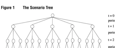
A scenario tree is illustrated in Figure 1. The nodes in the tree represent states of the world at a partic-ular point in time. In stochastic programming, deci-sions will be made at the nodes. The arcs represent realizations of the uncertain variables. The scenario tree branches off for each possible value of a
ran-dom vector x = x
1 x2 x1 in each stage t =
1 T. Note the difference from a decision tree which branches on both decisions and events.
2.2. The Scenario Generation Method
Figure 1 The Scenario Tree
Note. A path through the tree is called a scenario and consists of realizations of all random variables in all time periods.
with few (joint) outcomes, the generation of the tree is straightforward, as it can be done manually. How-ever, in all other cases, constructing the tree man-ually is practically impossible. Hence, we need a procedure for generating a scenario tree with the proper statistical properties. In some cases the spec-ified statistical properties partially describe a known underlying distribution, while in other cases the underlying distribution is unknown. In any case we denote our specifications as thespecified statistical prop-ertiesor thespecified distribution.
To present the model we introduce the following notation. Let S be the set of all specified statistical properties, andSVALi be the specified value of
statis-tical propertyi in S. Furthermore, let I be the num-ber of random variables,T be the number of stages, and Nt be the number of (conditional) outcomes in
stage t. In this presentation we assume, for simplic-ity, a symmetrical tree, meaning that the number of branches is the same for all conditional distributions in the same period. The tree in Figure 1 is symmet-rical with T=3, N1=5,N2=3, andN3=2. Define x
to be the outcome vector of dimension I·N1+I·N1·
N2+ · · · +I·N1·N2· · · · ·NT,p to be the probability vector of dimensionN1+N1·N2+ · · · +N1·N2· · · · ·
NT, and letfixpbe the mathematical expression for
statistical propertyiinS. LetMbe a matrix of zeroes and ones, whose number of rows equals the length of p and whose number of columns equals the number of nodes in the scenario tree, where each column is the indicator of a conditional distribution at one node. Each column inM extracts a conditional distribution in the scenario tree. Finally, let wi be the weight for statistical propertyiinS.
We want to construct x and p so that the sta-tistical properties of the approximating distribution
match (as well as possible) the specified statistical properties. We do this by minimizing a measure of distance between the statistical properties of the con-structed distribution and the specifications, subject to constraints defining the probabilities to be nonnega-tive and to sum up to one. For the rest of this paper, we shall use the square norm to measure distance. Of course, other choices are possible.
minxp
i∈S
wi·fixp−SVALi2
p·M=1 (1) p≥0
In this general description of the model, we let p be a variable in the optimization problem. We might also treatpas a parameter. See §4.1 for guidance with regard to this choice. Because of nonconvexities of the optimization problem, or inconsistent specifications, we might not obtain a perfect match. If this is the case, the weightswican incorporate the relative importance
of satisfying the different specifications, as well as the quality of (trust in) the data. Of course, the weights are only relevant if there exists a trade-off between some of the specifications, which means that not all specifications are perfectly satisfied.
Since the optimization problem (1) is generally not convex, the solution might be (and probably is) a local solution. But for our purposes it is satisfactory to have a solution with distribution properties equal to or close to the specifications—even if there might exist other and even better solutions. An objective value equal to or close to zero indicates that the distribu-tion of the scenarios has a perfect or good match with the specifications. To solve the problem, we apply a heuristic where we rerun the model from different starting points until a satisfactory match is obtained; see §§3.1 and 3.2 for details. For more sophisticated nonconvex optimization methods, see Horst and Tuy (1990), and the references therein.
Table 1 Percentiles of the Marginal Cumulative Distributions
0% 5% 25% 50% 75% 95% 100%
Cash 30% 32% 36 % 40% 50% 62% 70% Bonds 45% 48% 52% 58% 65% 74% 82% Domestic stocks −300% −250% 00% 85% 150% 250% 350% International stocks −350% −300% 00% 90% 150% 300% 400%
either be conditional on, or independent of, the out-comes in earlier periods. In addition to specifying the higher moments of the distribution, worst case out-comes can be included to ensure that extreme events are captured.
Consider an asset allocation problem where the sce-nario tree describes the uncertain returns in differ-ent asset classes. Empirical studies of stockmarkets have documented an effect called volatility clumping, meaning that a period with high volatility is likely to be followed by a new period of high volatility; see, for example, Billio and Pelizzon (1997) for details. To model this phenomenon, we would like the volatil-ity (standard deviation) of the nth period outcomes with a common extremen−1th period outcome to be higher than average. By letting thenth period stan-dard deviation be parametric in then−1th period outcome, this relation can be expressed in the model. The expected value, skewness, or other distribution properties can be state dependent in the same way.
The freedom to specify any desired property also leads to some possible pitfalls. A more detailed description of these pitfalls, and guidance on how to avoid them, are given in §4.1.
3. Generation of a Single- and a
Multiple-Period Scenario Tree
This section illustrates the scenario generation method by single- and multiple-period examples. We leave the discussion of what are the relevant statisti-cal properties for §4, and for now simply assume that the relevant properties are specified. The example is taken from finance and the problem is to find the opti-mal allocation of funds between main groups of asset classes. We assume that the decision-maker is to split the funds between cash, bonds, domestic stocks, and international stocks.3.1. Single-Period Scenario Tree
The specifications that follow apply to the single-period case and to the first single-period of the multisingle-period case in §3.2. For each individual asset class, we let the decision-maker specify his or her market views in terms of (subjective) percentiles for the marginal dis-tributions as shown in Table 1. Note that for cash and bonds the market views are in terms of expectations for the interest rate, while for stocks the expectations are given for the total return.
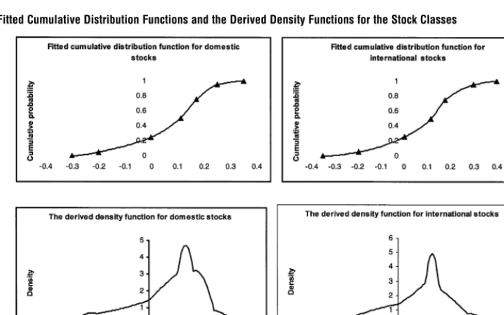
We fit an approximated cumulative distribution to the percentiles by using a NAG C library routine and derive the marginal distributions, as shown in Figures 2 and 3. The NAG C routine used for fitting the cumulative distribution does not guarantee that the second derivative changes in sign only once. This might cause a somewhat peculiar form of the density function.
Given the fitted cumulative distribution, we calcu-late the (central) moments. The example takes the first four moments into account. The decision-maker real-izes that extreme negative events influence the solu-tions, and specifies a worst-case event to be included in the scenarios. This can be done in several ways. Here we include a worst-case event where all asset classes move in the wrong direction at the same time, and we let the size of the move be propor-tional to the standard deviation. Table 2 summarizes all specifications of marginal distribution properties. The worst-case event for asset classiis generated by the following formula:WCi=Exi−F·SDxi, where
Figure 2 The Fitted Cumulative Distribution Functions and the Derived Density Functions for the Bond Classes
Note. Specified percentiles are marked with triangles.
[image:6.612.106.468.440.666.2]Table 2 Statistical Properties Derived from the Marginal Distributions in Figures 2 and 3
Expected Standard Worst-case value deviation event
(%) (%) Skewness Kurtosis∗ (%)
Cash 433 094 080 26 2 6 68 Bonds 591 082 049 239 796 Domestic stocks 76 1 1338 −075 293 −2584 International stocks 809 1570 −074 297 −3116
∗The normal distribution has a kurtosis of three. A kurtosis of less than
[image:7.612.45.288.291.368.2]three means that the distribution is less peaked around the mean than the normal distribution.
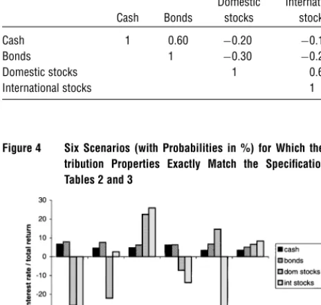
Table 3 Specification of Correlations
Domestic International Cash Bonds stocks stocks Cash 1 060 −020 −010
Bonds 1 −030 −020
Domestic stocks 1 060
International stocks 1
Figure 4 Six Scenarios (with Probabilities in %) for Which the Dis-tribution Properties Exactly Match the Specifications in Tables 2 and 3
Note.The worst-case event is given in the left-most scenario.
relevant. The correlations are estimated by empirical data, see Table 3.
A perfect match with the specifications in Tables 2 and 3 is obtained when the number of scenarios is six or higher. Due to the noncovexity of Problem (1), there are several possible distributions. One of these is given in Figure 4. See §4.1 for a more general dis-cussion of the necessary number of scenarios versus the number of specifications.
3.2. Multiperiod Scenario Tree
Expanding from one to several periods complicates the scenario generation in many ways, and in par-ticular implies that intertemporal dependencies need to be considered. In §2, we gave an example from finance and argued that the volatility for stocks depends on previous returns. Some statistical proper-ties are clearly state dependent, while others might be specified independently of the state.
In this example we have chosen the expected value and the standard deviation to be state dependent, while the other statistical properties are independent of the state. The volatility for asset class i in period
t >1 is modeled in the following way in order to capture the volatility clumping effect:1
SDxi t=VCi· xi t−1−Exi t−1
+1−VCi·SDAVxi t (2)
where VCi∈01 is the volatility clumping
param-eter (a high VCi leads to a large degree of
volatil-ity clumping), xi t is the outcome for asset class i in
periodt Exi tis the expected value for the outcome
in asset classiin period tand SDAVxi tis the
aver-age standard deviation for asset classiin periodt. We model a mean reversion effect for the two bond classes.2 The expected interest rate for bond classiat
the end of period t >1is given by
Exi t=MRFi·MRLi+1−MRFi·xi t−1 (3)
where MRFi ∈ 01 is the mean reversion factor
(a high MRFi leads to a large degree of mean rever-sion),MRLi is the mean reversion level, andxi tis the
interest rate for bond classiat the end of periodt. For stocks we assume that there is a premium in terms of higher expected return for taking more risk,
[image:7.612.48.280.314.535.2]Table 4 Specification of Market Expectations
Distribution (End of) (End of) (End of) Asset class property Period 1 Period 2 Period 3 Cash–duration three months expected value of spot rate 433% State dep State dep standard deviation 094% State dep State dep skewness 080 080 080 kurtosis 26 2 26 2 262 worst-case event 668% State dep State dep Bonds–duration six years expected value spot rate 591% State dep State dep standard deviation 082% State dep State dep skewness 049 049 049 kurtosis 239 239 239 worst-case event 796% State dep State dep Domestic stocks expected value total return 761% State dep State dep standard deviation 1338% State dep State dep skewness −075 −075 −075 kurtosis 293 293 293 worst-case event −2584% State dep State dep International stocks expected value total return 809% State dep State dep standard deviation return 1570% State dep State dep skewness −074 −074 −074 kurtosis 297 297 297 worst-case event −3116% State dep State dep
and let the expected total return for stockclass i in periodt be given by:
Exi t=rt−1+RPi·SDxi t (4) where rt is the risk-free interest rate (in this model
approximated by the cash interest rate) at the end of period t SDxi t is the specified standard deviation
on stockclassiin periodt, andRPt is a riskpremium
constant for periodt.
For Period 1 we assume the same set of specifi-cations as for the single-period case. For Periods 2 and 3 the expected values and the standard devi-ations are state dependent as illustrated, while the rest of the specifications are state independent and assumed to be equal to the specifications in the first period. Table 4 summarizes the marginal distribution properties. Table 3 is used for the state independent correlations in all three periods. The riskpremium constant in the stockpricing model, RPt, is set to 0.3 for t=12, and 3. We let the volatility clumping parameter, VCi =03 for all assets, the mean rever-sion factor, MRFi=02 for interest rate classes, and the mean reversion level, MRLi=40% and 58% for
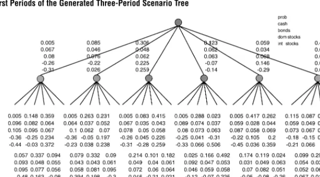
cash and bonds, respectively. A three-period tree that has a perfect match with the specifications in Tables 3 and 4 is generated. See Figure 5 for the outcomes in the two first periods.
Figure 5 The Two First Periods of the Generated Three-Period Scenario Tree
Note.The scenario tree has statistical properties that match the specifications in Tables 3 and 4.
Since the sequential approach requires the distribu-tion properties to be specified under each node in the tree, the approach lacks a direct control of the statis-tical properties defined overall outcomes in the later periodst >1. These properties are specified implic-itly by the other specifications and after constructing the tree, the decision-maker should analyze the gen-erated distribution to checkif his or her judgements can be trusted in this respect.
Also, the sequential approach involves a more rigid optimization scheme. Several first-period trees might satisfy the first-period specifications. Some of them might lead to conditional second-period specifications which make it impossible to obtain a full match, while others might lead to a full match in the second period. As opposed to the sequential approach, a model that constructs the whole tree in one large optimization is better in this regard, as the first-period trees that create difficulties are not feasible.
The main disadvantage with generating the whole tree in one large optimization is that the degree of nonconvexity increases, and a good or perfect match will be hard to construct. When the number of peri-ods grows, this will trigger the need for more sophis-ticated solution procedures.
In the example we produced a full match between the generated scenarios and the specifications. The tree was generated by solving the problem from a new set of starting values until a full match was
obtained. The choice of starting values should in general reflect the specified distributions. In this implementation we generated starting values for each random variable by sampling from uniform distribu-tions over an interval from −3 to +3 standard devi-ations, not taking the correlations into account. This crude approach worked well for the given example, and has proved successful for other cases as well. We have tested problems of up to five periods and approximately 8,000 scenarios, and it appears that the sequential procedure with the simple restart-heuristic leads to a full match if there are no inconsistencies in the specifications, and the tree is large enough.
With regard to solution times, the three-period tree of which two periods are shown in Figure 5, took63 seconds to generate on a Sun Ultra Sparc 1. Each single-period tree takes less than a second to construct.
4. Critical Success Factors
Section 4.2 raises the crucial question of what distri-bution properties should be matched.
4.1. Pitfalls in the Specifications
In §3 we saw that some of the statistical properties in later periods are derived from the outcomes in ear-lier periods. We denote thesederived specifications. The user should verify that the derived specifications are not implausible or contradictory. An example of the latter would be a conditional distribution in which one financial asset becomes first order stochastically dominant to another, creating an opportunity for arbi-trage in a later time period.
Implicit specifications mean that some statistical properties are specified implicitly by other specifica-tions. A simple example is the specification of means in one period being dependent on the outcome in the previous period, which implicitly specifies the correlation between periods. An implicit specification of a distribution property combined with a different explicit specification of the same property, will most likely lead to inconsistent specifications. The method can handle such inconsistencies, but there will of course be a trade-off between them. However, the decision-maker might not be comfortable with such a contradiction. Verification of implicit specifications and an understanding of how all the specifications relate are essential to avoid this.
Overspecifications means that the specifications are too extensive relative to the size of the scenario tree. Obvious examples are to specify a skewness (different from zero) or a correlation (different from minus one, zero, or one) for a discrete two point distribution with fixed probabilities.
If the number of scenarios is large relative to the requirements of the specifications, the problem is underspecified. The resulting scenario tree might satisfy the specifications but still have undesirable character-istics. Test examples have shown that in cases where the probabilities are defined as variables, underspec-ification leads to a solution where the extra degrees of freedom are used to produce zero probability out-comes. If the probabilities are fixed in an underspec-ified model, we typically observe that the scenarios that are not needed obtain outcomes of the random variables very close to their means. This might cause
problems if we wish to generate larger trees, and we shall see later in this section how to proceed in such cases. To avoid underspecifications, the number of specifications must be balanced relative to the size of the tree.
To understand when over and underspecifications occur, an analysis is made of the relationship between the characteristics of the specifications and the num-ber of outcomes necessary to obtain a perfect match. Consider a single-period problem where a continu-ous distribution of a single variable is to be approxi-mated by a discrete distribution. It is known (see for example Miller and Rice 1983 for a discussion) that the first 2·N−1 moments plus the requirement that the probabilities sum up to one, can be matched with
N points. In that case there are equally many vari-ables (outcomes and probabilities) as there are con-straints. The strength of this result lies in the fact that we get positive probabilities. As soon as we add extra requirements, this simple way of counting variables and constraints does not hold. But we may still use the idea of counting degrees of freedom to make a guess about the size of the tree.
As an example, take a five-dimensional case and specify the first four moments for each variable plus all correlations. The number of specifications is 30 (5 times 4 central moments plus 10 correlations). The number of variables in our tree in D+1·y−1, where D is the dimensionality of the problem (five in the example), and y is the number of outcomes. The minimum y that leads to 30 variables or more is 6. Although this rule of thumb may not always work, it seems to give a reasonable starting point for selecting the number of outcomes. In experiments working with power moments and correlations the authors have only very rarely needed to go above this minimal tree size. Of course, if inconsistencies are present, a perfect match can never be achieved, and we must simply lookfor a reasonable tree, at least so large that we do not face overspecification on top of inconsistencies.
that whether the probabilities are defined as vari-ables or parameters does not significantly influence the chance of obtaining a full match, despite the fact that the “degree of nonconvexity” increases when the probabilities are defined as variables as opposed to parameters.
4.2. Relevant Properties
In this section we show that the relevant statistical properties will depend on the characteristics of the problem at hand. For some problems, the relevant properties are easy to find, while for others they are harder. Our postulate is that if the relevant proper-ties are captured, all scenario trees that possess these properties will lead to approximately the same objec-tive function value when used in the decision model. With the help of this postulate, we provide guidance with respect to finding the relevant properties.
As an example of a case where it is easy to determine the relevant properties, consider a single-period mean-variance model with no legal or pol-icy constraints. The objective function can be written as a trade-off between the expected value and the variance:
max !·Ew−1−!·VARw
where !∈01 is a utility parameter determining the riskaversion and w is the uncertain wealth at the end of the planning period. For more details, see Markowitz (1959). For this model, all relevant proper-ties are captured in the first two moments, and differ-ent scenario trees with the same mean and covariance matrix will lead to identical solutions.
For the mean-variance model we knew in advance what were the relevant properties. For most decision problems, this is not the case. If we do not know the relevant properties, how do we find them? To illus-trate, we apply a model that was developed for a Norwegian life insurance company and is currently in use for actual decision making. A detailed descrip-tion of the model is given in Høyland and Wallace (1997). The objective is to maximize the riskadjusted portfolio value at the end of the planning period. For this analysis, a two-period (i.e., three-stage) version of that model is used, and, as in §3, four asset classes are introduced.
To find the relevant properties for this problem, we generate many different scenario trees with the same statistical properties and checkthe stability in the objective function values. If the stability is not good enough, we add new properties, and checkthe stability again. If the result is still not good enough, we can either continue adding statistical properties or we can use a sampling approach. If we sample, several different small trees (with the same statistical properties) are constructed and aggregated into one large tree. In other words, we sample a number of small trees and combine these small trees while pre-serving the specified statistical properties to create the large tree, which is the input to the optimization. By doing this we reduce the noise in the statistical prop-erties that are not specified. The following analyses show the effect of both adding statistical properties and the effect of sampling. We test for three sets of specifications with different characteristics. In Set 1 the correlation and the first and second moments of the marginal distributions are specified. In addition to the specifications of the first set, Set 2 includes specifications of the third and the fourth moments of the marginal distributions. Set 3 also includes a worst case outcomes. We generate two-period scenario trees as described in §3.2. The values of the statistical prop-erties that are specified are the same in all three sets, and given by Table 3 and by the specifications for the two first periods of Table 4. While Set 1 includes the two first moments of the specifications of Table 4, Set 3 includes all the specifications. We first gener-ate scenario trees with 30 outcomes in the first period and 6 outcomes in the second, obtained by aggre-gating 5 small trees with 6 outcomes in each period. Table 5 shows the stability of the objective function value for the three sets of specifications and we see that the stability improves as more statistical prop-erties are added. The stability in Set 3 is improved by more than 50% relative to Set 1. We see that the specification of the third and the fourth (marginal) moments has a large influence.
Table 5 Stability in the Objective Function Value for Three Different Sets of Specifications
Ex STD(x) High(x) Low(x) Set 1: EV, STDEV, CORR 11231 0384 11348 11151 Set 2: EV, STDEV, 11199 0203 11274 11147
SKEW, KURT, CORR
Set 3: EV, STDEV, 11198 0183 11248 11161 SKEW, KURT, CORR and
worst case outcomes
Note.For each specification set, 200 different scenario trees are generated, and 200 objective function valuesxsof the decision model are obtained.
The figures show the expected value and the standard deviation in addition to the highest and lowest objective function value for each specification set.
in the second period (i.e., 900 scenarios), using speci-fication Set 2. Solving the model for 60 different such scenario trees shows that the standard deviation in the objective value is reduced from 0.203 (refer to Table 5) to 0.100. For practical applications the sam-pling procedure has proved to be a good alterna-tive to adding statistics to match. In particular, higher that second order co-moments will be difficult for a decision-maker to quantify and they will also compli-cate the construction of the scenario tree by making the problem much harder to solve.
We have measured the quality of the scenario tree by the stability in the objective function value, not by the stability in the decision variables. Usually we will not require stability in the decisions. If the objective function value is “flat” with respect to changes the decisions, i.e., many different decision structures are approximately equally good, we might not achieve stability in the solutions even though we have sta-bility in the objective function value. However, we do not see this as a problem, but rather as a desir-able characteristic of the decision problem. The model above, though, is stable also in the decisions with respect to different scenario trees; see Table 6.
For the portfolio management model above, the relevant statistical properties seem to be captured by the first four central moments and the correla-tion matrix (all explicitly specified), and the sam-pling procedure which is applied to reduce the noise in the statistical properties which are not specified. It is hard to give a general characterization of rel-evant statistical properties and how to find them.
Table 6 Stability in the Decision Variables
Domestic Foreign Cash Bonds stocks stocks Average optimal portfolio 36777 93 94 Standard deviation in optimal 35 25 11 14
allocation
Note.The model is solved for 60 different two-period scenario trees of 900 scenarios generated by constructing and combining 25 small scenario trees with statistical properties as in Set 2.
As illustrated, the relevant properties depend on the objective function. With a quadratic utility function, the means and the variance/covariance matrix accu-rately determine the objective function. However, the relevant statistical properties will also depend on legal regulations, business environment, and self-proclaimed policy restrictions, i.e., on the constraints in the model. For instance, a portfolio management problem with a quadratic utility function in the pres-ence of capital adequacy constraints, solved for two different scenario trees with the same mean and variance/covariance, but different third and fourth moments, might lead to different optimal solutions.
5. Conclusions
In models of decision making under uncertainty it is essential to represent the uncertainties in a form suit-able for analysis. We have illustrated a method that generates a limited number of discrete scenarios that satisfy prespecified statistical properties. A single-period and a three-single-period scenario tree were gener-ated and the results illustrate the strengths of the method: The decision-maker was allowed to specify whatever distribution properties were found relevant, and a limited number of scenarios, with distribution properties that were consistent with the specifications, were generated.
The user should be aware of the possible pitfalls when specifying the statistical properties. We have drawn attention to derived, implicit, over and under-specifications, and discussed how to avoid these pitfalls. Further, we gave a simple formula as guid-ance for finding the smallest number of outcomes needed to obtain a perfect match.
[image:12.612.41.282.128.219.2]showed that this choice is problem dependent. We argued that these properties could be determined ex ante for some models, while for others they are harder or impossible to prescribe. The postulate we used to find the relevant properties in the difficult cases is that if different scenario trees, all possess-ing the same statistical properties, lead to the same objective function value in the decision model, then the relevant properties are captured in these trees. The paper also analyzed a multistage portfolio man-agement model. When solving the model for differ-ent scenario trees and matching the first four cdiffer-entral moments and correlations, the stability in the objec-tive function value was reasonably good. However, we showed that the stability was further improved by solving for larger scenario trees generated by aggre-gating many different small scenario trees. Hence, a combination of scenario construction and tree aggreg-ation leads to the best results.
Acknowledgments
This research is partly supported by Gjensidige Forsikring. The authors want to thankErikRanberg, Sjur Westgaard and Tore Andre Lysebo from Gjensidige for valuable discussions and con-tributions. Further, we want to acknowledge Amund Skavhaug at Norwegian University of Science and Technology for his help with the implementation and the debugging. Francesco A. Rossi at Uni-versitá di Verona deserves our gratitude for reading and comment-ing on an early version of the paper. They are also indebted to the associate editor and two referees.
References
Billio, M., L. Pelizzon. 1997. Pricing options with switching volatil-ity. Working paper 97.07, Department of Economics, University of Venice, Venice, Italy.
Cariño, D.R., T. Kent, D.H. Myers, S. Stacy, M. Sylvanus, A.L. Turner, K. Watanabe, W.T. Ziemba. 1994. The Russel-Yasuda Kasai model: An asset/liability model for a Japanese insurance company using multistage stochastic programming. Interfaces2429–49.
, D.H. Myers, W.T. Ziemba. 1998. Concepts, technical issues, and uses of the Russel-Yasuda Kasai financial planning model. Oper. Res.46450–462.
, W.T. Ziemba. 1998. Formulation of the Russel-Yasuda Kasai financial planning model.Oper. Res.46433–449.
Chen, Z., G. Consigli, M.A.H. Dempster, N. Hicks-Pedrón. 1997. Towards sequential sampling algorithms for dynamic port-folio management. Working paper 01/97, Finance Research Group, Judge Institute of Management Studies, University of Cambridge, UK.
Consigli, G., M.A.H. Dempster. 1996. Dynamic stochastic program-ming for asset-liability management. Working paper 04/96, Finance Research Group, Judge Institute of Management Stud-ies, University of Cambridge, UK.
Dupacová, J. 1996. Scenario based stochastic programs: Resistance with respect to sample.Ann. Oper. Res.6421–38.
Higle, J.L., S. Sen. 1991. Stochastic decomposition: An algorithm for two stage stochastic programs with recourse.Math. Oper. Res. 16650–669.
Horst, R., H. Tuy. 1990.Global Optimization.Springer-Verlag, Berlin, Germany.
Høyland, K. 1998. Asset liability management for a life insur-ance company—a stochastic programming approach. Ph.D. dissertation, Norwegian University of Science and Technology, Trondheim, Norway.
, S.W. Wallace. 1997. Analyzing the legal regulations in the norwegian life insurance business using a multi-stage asset liability management model. Eur. J. Oper. Res. To appear.
Infanger, G. 1994.Planning Under Uncertainty—Solving Large-Scale Stochastic Linear Programs.Boyd and Fraser Publishing Com-pany, MA.
Keefer, D.L. 1994. Certainty equivalents for three-point discrete-distribution approximations.Management Sci.40760–773. , S.E. Bodily. 1983. Three-point approximations for continuous random variables.Management Sci.29595–609.
Markowitz, H.M. 1959.Portfolio Selection: Efficient Diversification of Investment.Yale University Press, New Haven, CT.
Merkhofer, M.W. 1987. Quantifying judgmental uncertainty: Methodolgy, experiences and insights. IEEE Trans. Systems, Man, and Cybernetics760–773.
Miller, A.C., T.R. Rice. 1983. Discrete approximations of probability distributions.Management Sci.29352–362.
Smith, J.E. 1993. Moment methods for decision analysis. Manage-ment Sci.39340–358.
Spetzler, C.S., C.-A.S. Stael von Holstein. 1975. Probability encoding in decision analysis.Management Sci.22340–358.
Wang, J. 1995. Statistical inference for stochastic programming. Reports of the Institute of Mathematics–95.5, Nanjing Univer-sity, Nanjing 210008, Peoples Republic of China.
Zenios, S. 1995. Asset/liability management under uncertainty for fixed-income securities.Ann. Oper. Res.5977–97.
, M.S. Shtilman. 1993. Constructing optimal samples from a binomial lattice.J. Inform. Optim. Sci.14125–147.