Predictability of Equity Models

Predictability of Equity Models

Valls Pereira, Pedro L. and Chicaroli, Rodrigo

São Paulo School of Economics

January 2009

Online at

https://mpra.ub.uni-muenchen.de/10955/

PREDICTABILITY OF EQUITY MODELS

Rodrigo Chicaroli

Pátria Investimentos

Av. Brigadeira Faria Lima 2055 – 7

Floor

01452-001 São Paulo – Brazil

E-mail:

rodrigo.chicaroli@patriainvestimentos.com.br

Pedro L. Valls Pereira

EESP-FGV

Rua Itapeva 747 – 12

Floor

01332-000 São Paulo – Brazil

E-mail:

pedro.valls@fgv.br

ABSTRACT

In this study, we verify the existence of predictability in the Brazilian equity market.

Unlike other studies in the same sense, which evaluate original series for each stock,

we evaluate synthetic series created on the basis of linear models of stocks.

Following Burgess (1999), we use the “stepwise regression” model for the formation

of models of each stock. We then use the variance ratio profile together with a Monte

Carlo simulation for the selection of models with potential predictability. Unlike

Burgess (1999), we carry out White’s Reality Check (2000) in order to verify the

existence of positive returns for the period outside the sample. We use the strategies

proposed by Sullivan, Timmermann & White (1999) and Hsu & Kuan (2005)

amounting to 26,410 simulated strategies. Finally, using the bootstrap methodology,

with 1,000 simulations, we find strong evidence of predictability in the models,

including transaction costs.

Keywords: predictability, variance ratio profile, Monte Carlo simulation, reality check,

bootstrap, technical analysis

1. INTRODUCTION

The predictability of equity markets is one of the principal issues facing the

financial community and has been studied for several decades by academics and

market participants. Over time, various models and theories have been developed

and used for investment decision making, with the objective of obtaining strategies

with a positive expected return. At the same time, the significance of the results of

these models has been discussed since Fama & Blume (1966). Lo & MacKinley

(1995) sought indications of market inefficiencies through the so-called “maximally

predictable portfolios”. Lo & MacKinley (1990) had already highlighted the data

snooping effect, which deals with the problem arising from the exhaustive use of the

same data series, leading the studies to spurious results. Stock models were

suggested by Burgess (1999) to investigate the predictability of FTSE100 shares,

identifying models with greater predictability potential. Within Brazil, Baptista & Valls

Pereira (2006) investigated the performance of technical analysis on the intraday

data of the Bovespa index future, while Boainain & Valls Pereira (2007) tested the

head and shoulders pattern in the Bovespa spot market.

Unlike many studies, we analyzed the predictability of a synthetic price series,

constructed on the basis of formation of linear models. Such models are constructed

on the basis of the stepwise regression methodology. Following Burgess (1999), for

each stock analyzed, we arrived at a model with 5 regressors, the predictive potential

of which shall be evaluated by the criterion of variance ratio profile (VRP). Such

methodology is sufficient when applied directly to the original stock series. At the

same time, the models present a reversion to the mean bias created by construction,

using the stepwise regression methodology. In order to correct this bias, we carried

out a Monte Carlo simulation, in which the entire process of formation of models was

artificially generated on the basis of 1,000 generations of random walks, originating

observations on the variance ratio profile for each model. On the basis of this

distribution and a confidence level, we succeeded in identifying models with

predictability potential.

The second part of the study consists of the confirmation of the existence of

In the same way as Sullivan, Timmermann & White (1999) and Hsu & Kuan

(2005), we used White’s (2000) Reality Check methodology in order to overcome the

effect of data snooping on the results. According to this methodology, we created a

universe of 26,410 rules on the basis of 10 groups of strategies widely used by the

financial community. While this is a large number of rules, this number results from

many variations of a few simple rules. In order to carry out a more extensive test,

various more complex strategies, involving different indicators, could be included in

this universe. This is because, in practice, financial market operators rarely use

simple rules to obtain positive returns. In general they use sets of more complex rules

to give more precise operating signals.

Finally, we carried out a bootstrap simulation, with 1,000 observations, in order

to obtain the empirical distribution used to test the null hypothesis of the reality check,

and to conclude in favor of the existence of predictability in the created models.

This dissertation is organized in the following manner. In chapter 2, we present

the data used for the realization of the tests. In chapter 3, we describe a methodology

for the formation and selection of the models. In chapter 4, we present White’s (2000)

Reality Check methodology, used to test predictability without a data snooping bias.

In chapter 5, we present and discuss the results obtained, and finally, in chapter 6,

2. DATA

The daily price series used in this study were obtained from Economática. All

of the series were corrected for corporate events, such as dividends, splits and

subscriptions. The period covered by the study is equivalent to 2,147 days between

1/4/1999 and 28/8/2007, with this period divided into two sub-periods. The first from

1/4/1999 to 30/12/2003, containing 1,239 observations, was used for the formation

and selection of the models. This shall be termed the intra-sample model. The

second period, between 2/1/2004 and 28/8/2007, containing 908 observations, was

used to carry out the Reality Check, considering the period outside the sample.

The database for the study consists of 43 stocks traded on the São Paulo

stock exchange (Bovespa), a list of which is presented in the annexes to the study,

representing most of the volume traded on this stock exchange during the period.

The study excluded: stocks which cease to exist at any time during the period in

question; stocks which were not traded on any day of the period; stocks with an

average daily volume of less than 5 million Brazilian reais; and penny stocks, for

3. MODELS

Stock returns are generally influenced by two distinct risks. Specific risk,

relating to information on the stock itself and global risk, referring to information

affecting the equity market as a whole.

Various models have been presented over time with the objective of modifying

the original stock series, in order to remove the effects of global risk and explore the

predictable components of the assets in question. These models are termed

statistical arbitrage. According to Burgess (1999), statistical arbitrage is defined as

the generalization of the traditional “risk-free” arbitrage, in which two combinations of

assets with identical cash flows are constructed and any price discrepancies between

the two equivalent assets are explored. A portfolio consisting of the two combinations

(long + short) may be seen as a synthetic asset from which any divergence of the

price from zero may be seen as an arbitrage opportunity1.

According to the definition by Burgess (1999), we create synthetic assets from

each stock, amounting to 43 synthetic series. Each of the series is the result of a

price regression for the respective share, used as a dependent variable, against 5

regressors (stock prices), defined systematically by the stepwise regression process:

where RESs,t is the residue of the price model, Ps,t , for stock “s”, Pc(i,s ) is the price of

the i-th component of the same model and ws,i is the associated regression

coefficient.

Unlike Burgess (1999), we removed the constant regression term so that the

final result presented a price series which in practice was entirely simulated for an

investor. In this way, using 6 stocks with their respective weights, we can construct a

portfolio identical to those of the models without concern for the independent term.

information criterion possible. In the specific case, we used Akaike. At the end of the

process, we have the five regressors which best explain the price of the dependent

variable. We thus expected that the models generated would show stocks of the

same company or same sector as the regressors, since these are the stocks which

show the highest correlation and must be the most suitable to explain stock prices

seen as dependent variables.

3.1. Variance ratio profile

In order to identify which models present predictability potential, we need to

apply some type of stationarity test to the residues. In order to do this, we use the

variance ratio test, since it is a more powerful test with regard to alternative methods,

such as standard cointegration tests.

The principle of the variance ratio test follows from the fact that random walks

show linear variances with regard to the period over which the returns are measured.

In this way, the variance of the series of returns over days must be equal to times

the variance of the series of 1-day returns. In this way, as defined in Burgess (1999),

the variance ratio function is given by:

In the case of a random walk, the variance ratio formula must be equal to 1 for

any value of . Hence, in order to carry out the variance ratio test in the manner

presented, we need to choose some value for . Having said this, there is no

optimum value, leading us to make an arbitrary choice. In order to avoid this problem,

instead of using the discrete RV test, we use the variance ratio profile (VRP), which is

the function (2) for varying between 1 and 50.

Using the entire profile of this curve, we have another advantage. The VRP

provides us with information on the dynamics of the process. I.e., a positive VRP

gradient indicates positive autocorrelation and hence a trend in the series. On the

other hand, a negative gradient of the VRP indicates negative autocorrelation, and

hence a reversion to the mean or cyclical behavior.

In this way, our objective is to identify which models show a VRP which differs

from the unit profile, i.e., the profile of a random walk. Consequently, we shall identify

which models present some predictability potential.

3.2. Monte Carlo Simulation

The methodology presented so far presents two major problems. The first is

that we are carrying out the VRP test on a regression residue, and hence we shall

have a reversion to the mean bias, generated by construction. I.e. the residue of a

random walk regression will show a VRP of less than 1, which would invalidate the

test. The second problem is that we have a selection bias deriving from the choice of

5 regressors from a universe of 42, corresponding to the problem of data snooping

highlighted by Lo & MacKinley (1990).

In order to solve these problems, we carried out a Monte Carlo simulation in

order to create a distribution of variance ratio profile on models obtained on the basis

of random walks series. I.e. we created 43 series of random walks representing our

stock universe and applied the same selection methodology for models using

stepwise regression. For each model obtained, we calculated its variance ratio

profile. This procedure was repeated 500 times, amounting to 21,500 variance ratio

profiles which shall be used as a distribution for VRPs of random walks. In this way,

our objective is no longer to identify models with a VRP differing from unity, but

profiles which differ from the distribution encountered.

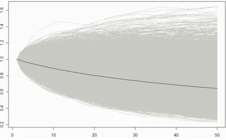
In Figure 1, we have the distribution of variance ratio profiles originated via the

stepwise regression methodology. The figure clearly highlights the bias introduced by

the method. We may clearly observe that the average profile shows considerable

downward divergence from the unit profile, indicating a reversion to the mean. At the

same time, we know that the profiles were all originated from random walks, and

hence cannot show any predictability.

In order to identify the divergence of the variance ratio profiles of each model

The Mahalanobis statistical distance between two points and

in a p-dimensional space is defined as:

where S is the correlation matrix and is the norm of x.

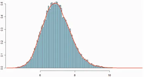
Figure 2 presents the distribution of Mahalanobis distances between each

VRP simulated by Monte Carlo and its average. This distribution, together with a

confidence level, shall be used to identify which models diverge from a random walk,

and hence have predictability potential for testing with the reality check.

(3)

4. REALITY CHECK

After having identified the models with predictability potential, our problem is to

test whether de facto, an investor succeeds in obtaining positive returns over the

period outside the sample. To do this, we must propose strategies to explore price

divergences of the creative models. A possible path is to propose a number of

strategies and to test them for the period outside the sample. At the same time, the

reuse of this data period may cause the problem of data snooping, highlighted by Lo

& MacKinley (1990).

In order to avoid this problem, we use the methodology used by White (2000),

Sullivan, Timmermann & White (1999) and Hsu & Kuan (2005), i.e. we implement the

reality check on a universe of technical analysis strategies which are extensively

discussed in the literature and among market operators.

4.1. White’s Reality Check

Considering as a measure of performance of the k-th strategy,

the null hypothesis of the test is that there is no strategy with a positive return within

the universe of M strategies:

In order for there to be predictability in the constructed models, we need to

reject the null hypothesis, indicating that there is at least one strategy with a positive

mean return. In this study, we use the mean daily return as a measure of

performance of strategies and carry out the tests on the maximum normalized mean

return, given by:

Where is the mean return of strategy k.

(4)

Following White (2000), we use the bootstrap methodology to determine the

p-value of . In order to do this, we carried out 1,000 iterations of the method in order

to arrive at the empirical distribution of , calculated in the following way:

.

Considering to be the matrix of daily returns n x M, where n=907 returns and

M=26,410 strategies, each stage of the bootstrap methodology consists of the

following steps:

1. Choose a line from the original matrix at random to be the first

line of the new matrix *.

2. The second line is selected at random from the original matrix

with probability p, or is defined as the next line to the one chosen in the

preceding step with a probability of (1-p). Like Sullivan,

Timmermann & White (1999) and Hsu & Kuan (2005), we used a probability of

p = 0.10.

3. Repeat step 2 until the new matrix *b is completed, corresponding to the b-th

bootstrap simulation2.

4.2. Universe of strategies

In order to carry out White’s reality check, it is fundamental for us to define a

broad universe of strategies. In this study, we adopt the same rules as those used by

Hsu & Kuan (2005) and Sullivan, Timmermann & White (1999).

Strategy Description Total

Sullivan, Timmermann & White (1999)

FR Filter Rules 497

MA Moving Averages 2,040 SR Support and Resistance 1,220

CB Channel 1,400

MSP Price Moment 1,760

Hsu & Kuan (2005)

OCO Head and Shoulders 1,200

TA Triangle 540

RA Rectangle 1,668

DTB Double Tops 2,160

BTB Inverted Triangle 720

Total 13,205

Contrary Rules 13,205

TOTAL 26,410

Table 1 presents the groups of strategies used for the formation of the

universe of rules. Strategies using volume as a decision variable were excluded,

since the constructed models do not contain information on volumes traded. All

parameters used in the universe of strategies may be consulted in the annexes to the

study. We present below a brief explanation of the groups of strategies used.

Filter Rules (FR)

According to the filter rule, a long position is opened when the price of an

asset increases by at least “x” percent. This position is maintained until the price falls

“x” percent relative to the last high, when simultaneously, we establish a short

position. In analogous fashion, the short position is closed when the price again rises

by “x” percent relative to the previous low, when we establish a new long position.

In addition, a number of variables are included in this model. Firstly, we have

two distinct definitions of the previous high and previous low. The first defines the

peaks relative to the duration of the last position. The second defines the peaks as

the maximum or minimum price over the interval of “e” days. We also consider the

strategy of maintaining the positions for a given constant period of “c” days, ignoring

any other signals during this period. And finally, we force the model to show periods

without a position, i.e. remaining out of the market, with the result that closures of

positions occur on the basis of a price movement of “y” percent relative to the last

peak, evidently considering that “y” must be less than “x”.3

This group contains a total of 497 strategies.

Moving Averages (MA)

According to the basic rule of moving averages, a long position is maintained

while the price remains above the moving average. As soon as the price falls below

this average, the investor's position is inverted. Once again, some alterations to this

rule are presented. More than one moving average may be used to generate buy and

sell signals. E.g. we use the crossing of two moving averages, with a long position

maintained while the short-term moving average is above the long-term moving

average. The inversion of position takes place when the moving averages cross. In

addition, two filters are used to avoid false signals. The first is a band multiplier,

which only generate signals when the crossing of prices exceeds “b” percent. The

remains valid for “d” days. Once again, we consider the strategy with a fixed number

of “c” days for maintaining each position.

This group contains a total of 2,040 strategies.

Support and Resistance (SR)

The principle of the rule of support and resistance is to buy when the price is

above the maximum of the last “n” days, and to sell when the price is below the

minimum of the last “n” days. Once again, we use an alternative definition of

maximum and minimum, i.e., we define a maximum (minimum) as the most recent

price which is higher than the prices of the last “e” days. In the same way as the

moving averages rule, we use a band filter, “b”, a lag filter, “d”, and also impose the

constraint that positions are maintained for a fixed number of “c” days.

This group contains a total of 1,220 strategies.

Channel (CB)

The channel rule, better known as a “channel breakout”, consists of

establishing long positions when the price is above the channel, and short positions

when the price is below it. A channel is formed when the maximum price over “n”

days is within “x” percent of the minimum of the “n” days. We also use the

parameters of “c” set days with a position and the “b” band filter.

Price Moment (MSP)

The moment strategy, extensively discussed in the literature and among

market participants, is based on a momentum oscillator such as the return over “m”

days, calculated at time t by

m t m t t t p p p R − − −

= , where p_t may be the closing price of the

series. We use three types of oscillator to generate signals. Firstly, we have the

simple oscillator, corresponding toR_t. Then we have the moving average oscillator,

which is the moving average of “m” days. And finally, we have the oscillator of

crossing of moving averages, based on the ratio between two moving averages of

“w1“ and “w2“ days on returns of “m” days, with “w1“ < “w2“. The rule is based on

constructing long positions as soon as the oscillator crosses above a certain level of

“k” percent. All positions are maintained for a fixed period of “f” days.

This group contains a total of 1,760 strategies.

Head and Shoulders

The head and shoulders rule is defined by a consecutive pattern of peaks and

troughs. This patent occurs over 5 periods of “m” days when we have sequence a

peak (left shoulder), a trough (left), a central peak (head), another trough (right) and

finally, another peak (right shoulder). When a head and shoulders pattern occurs, a

short position is established. For this, the following prerequisites are necessary: the

right and left shoulders, as well as the troughs must not differ by more than “x”

percent from each other; the maximum price of the head period must be greater than

all the other periods; the minimum prices of the head and shoulders must be greater

than the prices of the troughs; and the maximum price of the troughs must be less

than the prices of the other periods.

This rule provides three methods for liquidating positions. Firstly, we determine

a fixed number of “f” days with a position. Then we use a stop-loss of “r” percent. And

Triangle (TA)

Like the head and shoulders rule, the triangle rule depends on a pattern of

peaks and troughs. Once again, we define 5 sub-periods of “m” days, ordered from 1

to 5, represented by “Mi“. A triangle may take two patterns. In the first, “M1“,“M3“ and

“M5“ are peaks in which “M1“> “M3“ > “M5“, and “m2” and “m4”are troughs in which

“m2” < “m4”. In the second pattern, “m1”, “m3” and “m5” are troughs for which “m1” <

“m3” < “m5” and, “M2” and “M4” are peaks for which “M2” > “M4”. In addition, the

minimum (maximum) price of a peak must be greater than the minimum (maximum)

price of a subsequent trough.

As soon as a triangle is identified, a long position is initiated as soon as the

price exceeds the last peak by “x” percent, or a short position is initiated when the

price falls by more than “x” percent from the last trough. Once again, three methods

are used for liquidating positions: “f” set days; stop-loss of “r” percent; and a filter with

“d” days.

This group contains a total of 540 strategies.

Rectangle (RA)

The rectangle rule is similar to the triangle rule, albeit with the alteration of the

criteria for formation of the figure. A rectangle is formed when the peaks “M1“,“M3“

and “M5“ (or “M2” and “M4”) are aligned on an upper horizontal line, and the troughs

“m2” and “m4” (or “m1”, “m3” and “m5”) also lie on a lower horizontal line. We say

prices are aligned when the difference between the maximum and minimum lies

within a band of “k” percent. After defining a rectangle, the same triangle rules are

applied for buy and sell signals. This group contains a total of 1,668 strategies.

Double Tops (DTB)

The rule for double tops is characterized by two patterns: two peaks or two

characterized when the periods “M1” and “M3” form a top relative to “m2”, and a

double bottom is formed when “m1” and “m3” form a trough relative to “M2”. A pattern

is identified if the sub-periods 1 and 3 show prices within a band of “k” percent. In

addition, the minimum (maximum) price of sub-period 2 must be at least “g” percent

lower (higher) than the average of the prices of the peaks (troughs), and the

minimum price (maximum) of a peak must be greater than the minimum (maximum)

of the subsequent trough. A long position is initiated when the price exceeds the last

peak by “x” percent. Once again, we use the three rules for liquidating positions: set

days “f”, stop-loss “r“ and filter of day “d”.

This group contains a total of 2,160 strategies.

Inverted Triangle (BTB)

The inverted triangle rule is identical to the triangle rule as presented, except for the

direction of convergence of the figure. The regular triangle shows a pattern of

convergence of peaks and troughs, while the inverted triangle shows a pattern of

divergence. In this way, the inverted triangle is defined when “M1”< “M3” < “M5” with

“m2” > “m4”, or “m1” > “m3” > “m5” with “M2” < “M4”.

5. RESULTS

5.1. Formation of models

All development of the stage of forming models and Monte Carlo simulations

was programmed in R, with the aid of a database in Access.

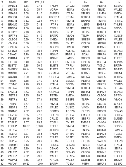
Table 2 presents the results obtained in the first stage of the study. For each

one of the 43 stocks analyzed, the stepwise regression procedure determined the 5

component shares of each model, defined as Ci. The components of each model are

presented by order of significance, with C1 as the asset which best explains the

prices of the stock in question.

As expected, we may verify in the table that the models of companies with two

classes of share, whether preferred or common, or which have a holding and an

operational company, always show the corresponding share as the most significant.

Evidently, since the two shares represent the same company, the values of shares

must have a greater correlation than with the rest of the market. These are: BRAP4

with VALE5, BRTP3 with BRTP4, ELET3 with ELET6, GOAU4 with GGBR4, ITAU4

with ITSA4, PETR3 with PETR4, TCSL3 with TCSL4, TNLP3 with TNLP4 and VALE3

with VALE54.

In addition, the results show us that in the majority of cases, the models of

companies with only one class of share have a share from the same sector as the

principal component. Once again, as expected, shares from the same sector should

present a greater correlation than with the rest of the market. Some examples are:

ARCZ6 with VCPA4, BBDC4 with UBBR11, BRKM5 with PTIP4, CLSC6 with CMIG4,

CSNA3 with USIM5, TLPP4 with BRTP3 and VIVO4 with BRTP4.

Table 2 also presents the Mahalanobis distance for the variance ratio profile of

the models relative to the average of the VRP for models simulated by Monte Carlo

methods. This distance, together with the empirical distribution illustrated by Figure 2,

indicates to us how each model diverges from a random walk. Hence, a confidence

level is sufficient to define which models show predictability potential. Table 2

presents the percentiles of the distances in the empirical distribution. Above 90%, we

have 30 models with predictability potential, corresponding to 70% of the models.

Above 95%, we have 26 models (60%). Above 99%, 14 models (33%) are selected,

while this number falls to 4 models (9%) when we use a percentile of 99.9%.

In order to select models with predictability, we use the 99% percentile. We

then have 14 models to realize White’s reality test and to verify whether the

predictability is confirmed for the period outside the sample. The selected models are

Ci Components

# Model Dm Pct (%) C1 C2 C3 C4 C5

1 AMBV4 8.64 97.3 TNLP4 CRUZ3 ITAU4 PETR3 SBSP3 2 ARCZ6 8.42 95.7 VCPA4 SDIA4 CMIG4 TBLE3 VALE5 3 BBAS3 8.08 91.6 EMBR3 ITSA4 CRUZ3 LAME4 CMIG4 4 BBDC4 8.96 98.7 UBBR11 ITSA4 BRTO4 SUZB5 ITAU4 5 BRAP4 7.44 74.1 VALE5 VIVO4 CSNA3 TNLP3 BBDC4 6 BRKM5 6.95 51.8 PTIP4 SDIA4 USIM5 EMBR3 TNLP3 7 BRTO4 7.56 78.4 TRPL4 BRTP4 BRTP3 KLBN4 BBDC4 8 BRTP3* 9.48 99.6 BRTP4 TNLP3 TLPP4 BRTO4 CPLE6 9 BRTP4 6.03 11.9 BRTP3 VIVO4 TNLP4 BRTO4 CLSC6 10 CLSC6 6.99 53.9 CMIG4 SBSP3 SUZB5 BRTP4 VALE3 11 CMIG4 6.86 47.3 CLSC6 TNLP4 CPLE6 ARCZ6 BBAS3 12 CPLE6 7.65 81.2 SBSP3 CMIG4 PTIP4 BRKM5 ELET3 13 CRUZ3 8.79 98.1 TLPP4 AMBV4 SUZB5 TBLE3 BBAS3 14 CSNA3* 9.70 99.8 USIM5 UBBR11 SDIA4 BRAP4 VALE3 15 DURA4 7.32 69.5 USIM5 LAME4 SBSP3 KLBN4 ELET6 16 ELET3 8.40 95.6 ELET6 EMBR3 CPLE6 BBDC4 SUZB5 17 ELET6* 9.88 99.9 ELET3 TRPL4 DURA4 TCSL3 BRTP4 18 EMBR3* 10.44 100.0 ELET3 TCSL3 SUZB5 TBLE3 BBAS3 19 GGBR4 7.71 83.2 GOAU4 VCPA4 BRKM5 TCSL4 SDIA4 20 GOAU4 8.00 90.1 GGBR4 LAME4 KLBN4 VALE5 BRTP4 21 ITAU4 8.58 97.0 ITSA4 BBDC4 PETR3 UBBR11 VALE3 22 ITSA4* 9.10 99.1 ITAU4 BBDC4 BBAS3 SUZB5 BRKM5 23 KLBN4 8.43 95.8 GOAU4 VIVO4 BRTO4 SUZB5 DURA4 24 LAME4 8.54 96.6 GOAU4 TLPP4 DURA4 BRKM5 BBAS3 25 PETR3 7.95 89.0 PETR4 AMBV4 DURA4 CLSC6 BRTO4 26 PETR4 8.61 97.1 PETR3 SBSP3 TLPP4 CPLE6 VIVO4 27 PTIP4 7.67 81.8 VIVO4 BRKM5 TLPP4 SUZB5 CPLE6 28 SBSP3 6.61 34.6 CPLE6 CLSC6 VIVO4 EMBR3 SDIA4 29 SDIA4* 9.82 99.8 BRKM5 ARCZ6 ELET3 SBSP3 CSNA3 30 SUZB5 8.65 97.3 CRUZ3 PTIP4 EMBR3 CLSC6 BBDC4 31 TBLE3* 10.16 99.9 CRUZ3 EMBR3 SBSP3 ARCZ6 SUZB5 32 TCSL3* 9.57 99.7 TCSL4 TNLP3 EMBR3 CMIG4 UBBR11 33 TCSL4* 10.67 100.0 TCSL3 VIVO4 TRPL4 TNLP4 BBDC4 34 TLPP4 8.81 98.2 BRTP3 PTIP4 TNLP4 CRUZ3 LAME4 35 TNLP3 8.87 98.4 TNLP4 BRTP3 PETR4 BRKM5 TCSL3 36 TNLP4* 9.23 99.3 TNLP3 BRTP4 TLPP4 AMBV4 CMIG4 37 TRPL4 8.25 93.9 BRTO4 TCSL4 ELET6 VALE3 CRUZ3 38 UBBR11 7.13 61.1 BBDC4 CSNA3 TCSL3 CMIG4 ITAU4 39 USIM5* 9.30 99.4 CSNA3 DURA4 BRKM5 KLBN4 SDIA4 40 VALE3* 9.82 99.8 VALE5 CSNA3 CLSC6 BRKM5 TRPL4 41 VALE5* 9.52 99.6 VALE3 BRAP4 CRUZ3 DURA4 TCSL4 42 VCPA4 8.15 92.6 ARCZ6 VALE5 GGBR4 BRTO4 USIM5 43 VIVO4* 10.63 100.0 BRTP4 TCSL4 PTIP4 BRAP4 SBSP3

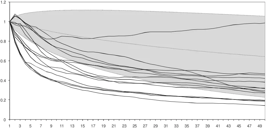
Figure 3 illustrates the variance ratio profile of the 14 selected models with

predictability potential, and presents the area in which the VRP of random walks

generated by the Monte Carlo simulation are concentrated, corresponding to the grey

area of the graph. This area was defined as the interval containing from 1% to 99% of

the simulated distribution. As we may observe, the VRP of the models are

concentrated below the random walks region, indicating that the models show a

reversion to the mean. Some models may be found outside the region, since, in

addition to its position, the Mahalanobis distance takes the entire format of the curve

into consideration. In this way, a curve with a format different from the average of

random walks may show a sufficiently large Dm to be considered as non-random.

0 0.2 0.4 0.6 0.8 1 1.2

1 3 5 7 9 11 13 15 17 19 21 23 25 27 29 31 33 35 37 39 41 43 45 47 49

5.2. Reality Check

In order to carry out the second stage of the study, i.e. to test for the

predictability of models created in the previous stage, we carried out 26,410

simulations during the period outside the sample between 2/1/2004 and 28/8/2007,

containing 908 observations. The simulations correspond to all combinations of rules

and parameters of the universal strategies described in section 4.1, the values of

which are presented in the annexes to this study.

We did not use the residue of the models for taking decisions on strategies

directly, but the ratio of prices of the models given by:

∑

Using the ratio of the models, we may interpret the series as the price of a

synthetic asset, with the purchase of this ratio equivalent to buying the principal asset

and selling the regressors5. The series were generated with the aid of Excel and the

simulations of the strategies carried out with the aid of WealthLab, a software

application which provides a suitable environment for the development of strategies.

All of the simulations were carried out in such a way that an investor would be

fully able to reproduce the strategies in the actual market. This is relevant, since

studies are frequently encountered in the literature which concentrate most of their

efforts on the theory and modeling statistical phenomena, while making little effort for

the tests of practical simulation. In general, rules are suggested which are naïve or

which do not take into consideration the operational problems of realizing such

strategies in a real market. Burgess (1999), for example, bases his results on a

simple regression of the innovation of the residual against certain lag levels and

differences. This type of test, common in studies in the field, does not consider e.g.

restrictions on executing orders at the close of the session. The regression in

question allows us to predict the returns for the next day on the basis of the

information at the close of trading. At the same time, there is a strong hypothesis that

the investor will execute the orders at the actual close on which the price for taking

5

his decision depends. In addition, the test requires that the investor always has an

open position in the market, a situation which may not be viable when all of the

transaction costs involved are taken into consideration.

In order to overcome these problems, all of the simulations realized in the

reality check were defined in such a way that the investor uses all of the available

information on the current day to operate in the market only on the following day. This

allows the investor to become aware before the market opening of all of the

operations to be realized during the day in question. In addition, all of the price series

used in this study are based on average daily prices. This allows the investor to have

much greater available liquidity than the execution at the closing prices, given that

the order is executed over the entire duration of the trading session. Nowadays, this

is viable, given the many algorithms which use electronic operations to determine the

average price of shares over a given period. These algorithms, known as VWAP or

TWAP, are already offered to investors by various brokers and information systems.

The transaction costs are not common to all market participants, and hence,

we decided to carry out two simulations. The first, without considering costs, and the

second, considering a cost of 0.10% of the financial volume of each operation. In this

way, each participant may evaluate how his cost structure may impact results.

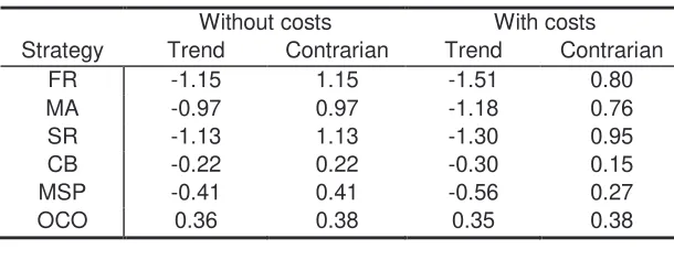
Table 3 presents the adjusted average returns6 of the strategies grouped by

type of rule used. We observe that the returns on strategies termed contrarian, i.e.,

which are the opposite of the original trend strategies, show positive returns. Without

transaction costs, we have an adjusted return of 0.55%, while with costs, we still

have a positive return of 0.45%. This result was expected since the variance ratio

profiles all fell below the region of the random walk, a fact which, as stated above,

indicates reversion to the mean.

Without costs With costs Strategy Trend Contrarian Trend Contrarian

TA 0.34 0.32 0.34 0.32 RA 0.34 0.38 0.34 0.38 DTB 0.33 0.15 0.32 0.14 BTB 0.34 0.37 0.34 0.37 Mean -0.22 0.55 -0.31 0.45

The maximum normalized average returns ( ) found were:

   = costs with 3.4% costs without % 8 . 3 n V

At the same time, while we have a strategy indicating a positive return, even

considering transaction costs, according to White (2000), we cannot conclude our

study without considering the effects of data snooping. This arises from the fact that

we are reusing the same period outside the sample to simulate different strategies.

Using the bootstrap methodology, with a probability p of 10%, we create the

empirical distribution of pursuant to (6). Figure 4 and Figure 5 present the

distributions obtained without and with transaction costs respectively.

0% 10% 20% 30% 40% 50% 60% 70% 80% 90% 100% 0 20 40 60 80 100 120

Table 3 – Table of the return (%) on groups of strategies

(8)

0% 10% 20% 30% 40% 50% 60% 70% 80% 90% 100%

0 20 40 60 80 100 120

We may observe that the values obtained in the distributions are all less than

the values of obtained from the series outside the sample, presented in (8). This is

equivalent to a very low p-value and leads us to conclude that we should reject the

null hypothesis (4) which states that there is no strategy with a positive return among

the M strategies. We thus arrive at the conclusion that it is possible for an investor to

obtain positive returns using the stock models presented.

6. CONCLUSION

In this study, we use the methodology used by Burgess (1999), for the

formation of statistical stock models applied to the Brazilian market, with the objective

of verifying the existence of predictability in this market. We found 14 models with

predictability potential according to the criterion of variance ratio profile, together with

a Monte Carlo simulation used to create an empirical distribution of the distances of

the VRPs of the random walk models. On the basis of the 14 models selected,

following Hsu & Kuan (2005) and Sullivan, Timmermann & White (1999), we carried

out White’s (2000) reality check in order to verify the predictability for the period

outside the sample. The tests were carried out in such a way that the investor is able

to reproduce all of the strategies in the actual market. The tests indicated to us a

number of groups of strategies with a positive return, even considering transaction

costs. As expected from the variance ratio profile, strategies which exploit reversion

to mean prices were those which presented the best results. In addition, we rejected

the null hypothesis of the test that there is no strategy with a positive return on a

universe of N strategies through the empirical distribution of , obtained by the

bootstrap methods. In so doing, we were able to verify strong indications of

predictability in the Brazilian equity market, using rules which may easily be

7. REFERENCES

BAPTISTA, R.F.F.; VALLS PEREIRA, P.L. Análise de Performance de Regras de

Análise Técnica Aplicada ao Mercado Intradiário do Futuro do Índice Bovespa [Analysis of Performance of Rules of Technical Analysis applied to the Intraday Bovespa Index Futures Market]. Ibmec São Paulo, 2006.

BOAINAIN, P.G.; VALLS PEREIRA, P.L. Ombro-Cabeça-Ombro: Testando a

lucratividade do padrão gráfico de análise técnica no mercado de ações brasileiro. [Head and Shoulders: Testing the Profitability of the Graphic Pattern of Technical Analysis in the Brazilian Equity Market] Anais do 70 Encontro

Brasileiro de Finanças. SBFin: São Paulo, 2007.

BURGESS, A. N. Statistical Arbitrage Models of the FTSE 100. In:Abu-Mostafa et al.

Computational Finance 99, MIT Press, Cambridge, 1999. p. 297-312.

FAMA, E.; BLUME, M.E. Filter Rules and Stock Market Trading. Journal of

Business 39, p. 226-241, 1966.

HSU, P.H.; KUAN, C.M. Re-Examining the Profitability of Technical Analysis

with White's Reality Check and Hansen's SPA Test. Available in SSRN:

<http://ssrn.com/abstract=685361>. Accessed in March 2005.

LO, A.W.; MACKINLAY, A.C. Data snooping Biases in Tests of Financial Asset

Pricing Models. Review of Financial Studies, v. 3, p. 431-467, 1990.

LO, A.W.; MACKINLAY, A.C. Maximizing predictability in the stock and bond

markets. In: LO, A.W.; MACKINLAY, A.C. A Non-Random Walk Down Wall Street,

Princeton University Press, New Jersey, 1995. p. 249-284.

WHITE, H. A Reality Check for Data Snooping. Econometrica 68, p. 1097-1126,

8. ANNEXES

8.1. Parameters used in the strategies

Filter rules (FR)

“x“ = 0.005, 0.01, 0.015, 0.02, 0.025, 0.03, 0.035, 0.04, 0.045, 0.05, 0.06, 0.07, 0.08,

0.09, 0.10, 0.12, 0.14, 0.16, 0.18, 0.20, 0.25, 0.30, 0.40, 0.50 (24 values);

“y“ = 0.005, 0.01, 0.015, 0.02, 0.025, 0.03, 0.04, 0.05, 0.075, 0.10, 0.15, 0.20 (12

values);

“e“ = 1, 2, 3, 4, 5, 10, 15, 20 (8 values);

“c“ = 5, 10, 25, 50 (4 values).

Moving Averages (MA)

“n“ = 2, 5,10, 15, 20, 25, 30, 40, 50, 75, 100, 125, 150, 200, 250 (15 values);

“b“ = 0.001, 0.005, 0.01, 0.015, 0.02, 0.03, 0.04, 0.05 (8 values);

“d“ = 2, 3, 4, 5 (4 values).

Support and Resistance (SR)

“n“ = 5, 10, 15, 20, 25, 50, 100, 150, 200, 250 (10 values);

“e“ = 2, 3, 4, 5, 10, 20, 25, 50, 100, 200 (10 values);

“b“ = 0.001, 0.005, 0.01, 0.015, 0.02, 0.03, 0.04, 0.05 (8 values);

“d“ = 2, 3, 4, 5 (4 values);

Channel (CB)

“n“ = 5, 10, 15, 20, 25, 50, 100, 150, 200, 250 (10 values);

“x“ = 0.005, 0.01, 0.02, 0.03, 0.05, 0.075, 0.10, 0.15 (8 values);

“b“ = 0.001, 0.005, 0.01, 0.015, 0.02, 0.03, 0.04, 0.05 (8 values);

“c“ = 5, 10, 25, 50 (4 values).

Price Moment (MSP)

“m“ = 2, 5, 10, 20, 30, 40, 50, 60, 125, 250 (10 values);

“w“ = 2, 5, 10, 20, 30, 40, 50, 60, 125, 250 (10 values);

“k“ = 0.05, 0.10, 0.15, 0.20 (4 values);

“f“ = 5, 10, 25, 40 (4 values).

Head & Shoulders

“n“ = 5, 10, 20, 50 (4 values);

“x“ = 0.005, 0.01, 0.015, 0.03, 0.05 (5 values);

“k“ = 0, 0.005, 0.01, 0.02, 0.03 (5 values);

“f“ = 5, 10, 25, 50 (4 values);

“r“ = 0.005, 0.0075, 0.01, 0.015 (4 values);

“d“ = 0.25, 0.5, 0.75, 1 (4 values).

Triangle (TA)

“n“ = 5, 10, 20, 50 (4 values);

“x“ = 0, 0.001, 0.003, 0.005, 0.0075, 0.01, 0.02, 0.03, 0.04, 0.05, 0.06, 0.07, 0.08,

0.09, 0.10 (15 values);

“f“ = 5, 10, 25, 50 (4 values);

“d“ = 2, 3, 4, 5 (4 values).

Rectangle (RA)

“n“ = 5, 10, 20, 50 (4 values);

“k“ = 0.005, 0.0075, 0.001 (3 values);

“x“ = 0, 0.001, 0.003, 0.005, 0.0075, 0.01, 0.02, 0.03, 0.04, 0.05, 0.06, 0.07, 0.08,

0.09, 0.10 (15 values);

“f“ = 5, 10, 25, 50 (4 values);

“r“ = 0.005, 0.0075, 0.01, 0.015 (4 values);

“d“ = 2, 3, 4, 5 (4 values).

Double Tops (DTB)

“n“ = 20, 40, 60 (3 values);

“k“ = 0.005, 0.01, 0.015, 0.03, 0.05 (5 values);

“g“ = 0.10, 0.15, 0.20 (3 values);

“x“ = 0, 0.01, 0.02, 0.03, (4 values);

“f“ = 5, 10, 25, 50 (4 values);

“r“ = 0.005, 0.0075, 0.01, 0.015 (4 values);

“d“ = 2, 3, 4, 5 (4 values).

Inverted Triangle (BTB)

“n“ = 5, 10, 20, 50 (4 values);

“x“ = 0, 0.001, 0.003, 0.005, 0.0075, 0.01, 0.02, 0.03, 0.04, 0.05, 0.06, 0.07, 0.08,

0.09, 0.10 (15 values);

“f“ = 5, 10, 25, 50 (4 values);

“r“ = 0.005, 0.0075, 0.01, 0.015 (4 values);

8.2. Stock tickers used

Ticker Company

AMBV4 AMBEV PN ARCZ6 ARACRUZ PNB BBAS3 BRASIL ON BBDC4 BRADESCO PN BRAP4 BRADESPAR PN BRKM5 BRASKEM PNA BRTO4 BRASIL TELEC PN BRTP3 BRASIL T PAR ON BRTP4 BRASIL T PAR PN CLSC6 CELESC PNB CMIG4 CEMIG PN CPLE6 COPEL PNB CRUZ3 SOUZA CRUZ ON CSNA3 SID NACIONAL ON DURA4 DURATEX PN

ELET3 ELETROBRAS ON ELET6 ELETROBRAS PNB EMBR3 EMBRAER ON GGBR4 GERDAU PN GOAU4 GERDAU MET PN

ITAU4 ITAUBANCO PN ITSA4 ITAUSA PN KLBN4 KLABIN S/A PN LAME4 LOJAS AMERIC PETR3 PETROBRAS ON PETR4 PETROBRAS PN PTIP4 IPIRANGA PET PN SBSP3 SABESP ON

SDIA4 SADIA S/A PN SUZB5 SUZANO PAPEL PNA TBLE3 TRACTEBEL ON TCSL3 TIM PART S/A ON TCSL4 TIM PART S/A PN TLPP4 TELESP PN TNLP3 TELEMAR ON TNLP4 TELEMAR PN TRPL4 TRAN PAULIST PN UBBR11 UNIBANCO UNT

USIM5 USIMINAS PNA VALE3 VALE R DOCE ON VALE5 VALE R DOCE PNA VCPA4 V C P PN