Deterministic randomness in a model of finance and growth

Deterministic randomness in a model of

finance and growth

Gomes, Orlando

Escola Superior de Comunicação Social - Instituto Politécnico de

Lisboa

February 2007

Online at

https://mpra.ub.uni-muenchen.de/2888/

Deterministic Randomness in a

Model of Finance and Growth

Orlando Gomes

∗

Escola Superior de Comunicação Social [Instituto Politécnico de Lisboa] and Unidade de Investigação em Desenvolvimento Empresarial [UNIDE/ISCTE].

- February, 2007 -

Abstract: Following the literature on growth, cycles and financial development, this paper

develops an endogenous growth model where the source of endogenous business cycles relates to the allocation of credit between productive investment and consumption. An important role is given to consumer sentiment, because this determines the willingness of households in terms of demand for credit; in particular, optimistic beliefs about the economy’s macro performance deviate financial resources from investment in favour of consumption. The dynamic analysis indicates that Neimark-Sacker and flip bifurcations eventually separate stable and unstable manifolds, and as a result a region of nonlinear motion is generated: cycles of various periodicities and chaotic motion characterize the behaviour of the long run time paths of accumulated wealth, output and consumption.

Keywords: Financial development, Endogenous business cycles, Endogenous growth,

Credit to consumption, Local bifurcations, Nonlinear dynamics, Chaos.

JEL classification: O16, E32, C62.

∗ _{Orlando Gomes; address: Escola Superior de Comunicação Social, Campus de Benfica do IPL,}

1549-014 Lisbon, Portugal. Phone number: + 351 93 342 09 15; fax: + 351 217 162 540. E-mail:

[email protected].

1. Introduction

Borrowing constraints have a relevant impact on growth and cycles. This

evidence has been studied, both in theoretical and empirical grounds, by a large group

of economists, from which we can highlight the contributions of Bernanke and Gertler

(1989), Kyotaki and Moore (1997), Levine (1997, 2005), Aghion, Banerjee and Piketty

(1999) and Amable, Chatelain and Ralf (2004), among others. Recently, some authors

have pointed to the idea that, under meaningful and reasonable assumptions, a

prototype growth-finance model is able to generate endogenous business cycles; this is

the path followed by Aghion, Baccheta and Banerjee (2004) and Caballé, Jarque and

Michetti (2006). Mostly in this last paper, the idea is to establish a link between credit

constraints or the level of financial development of an economy and the literature on

deterministic cycles first addressed in the early 1980s [e.g., Benhabib and Day (1981),

Day (1982), Boldrin and Montrucchio (1986), Deneckere and Pelikan (1986)] and

relaunched with the work by Christiano and Harrison (1999), who adapt a deterministic

version of the real business cycles model (RBC) to a scenario of endogenous

fluctuations by including in the setup an externality over the production of physical

goods that allows to consider an aggregate production function exhibiting increasing

returns to scale.

Endogenous cycles have been a strong source of motivation for recent

macroeconomic literature. Several directions are being followed. See, for instance,

Schmitt-Grohé (2000) and Guo and Lansing (2002), who also focus on the RBC setup,

Boldrin, Nishimura, Shigoka and Yano (2001), Mitra, Nishimura and Sorger (2005),

and related literature, who search for extreme conditions in which competitive markets

generate nonlinear motion, Cellarier (2006), who introduces a learning mechanism into

the growth setup to trigger chaotic motion, and Cazavillan, Lloyd-Braga and Pintus

(1998), Aloi, Dixon and Lloyd-Braga (2000), Lloyd-Braga, Nourry and Venditti

(2006), and related literature, where the search for endogenous cycles is based on the

OLG framework in the tradition of Grandmont (1985). For a survey on nonlinear

dynamics in macroeconomics see Gomes (2006).

In this paper, we follow on the footsteps of the work on financial constraints and

endogenous cycles, by proposing a model of endogenous growth (of the AK type) that

considers not only a constraint over credit, but also two alternatives concerning the

between borrowing to invest or borrowing to consume. The shares of credit directed to

one or to the other use are assumed as constant values if the economy performs as

expected (i.e., if the accumulated level of wealth follows a predefined trend).

Deviations from this expected performance are accounted by the representative agent,

who rises the share of credit to consumption when levels of wealth are above the

predicted outcome. In other words, consumer sentiment counts in what concerns how

the economy splits the available credit into the possible utilizations.

The previous ingredients allow to develop a growth model where, from a local

dynamic analysis point of view, bifurcations separating regions of stability and

instability are observable, and from a global dynamics perspective we find, for some

arrays of parameter values, the presence of cyclical and chaotic motion characterizing

the time evolution of the economic aggregates we consider: wealth (the central variable

for which the analysis is conducted) and, also, output, capital, investment, consumption

and even the share of credit allocated to each available use (since all these variables are

dependent on the path of wealth).

The remainder of the paper is organized as follows. Section 2 describes the

model. Sections 3 and 4 respect to the stability analysis, which is undertaken both

locally and globally. Section 5 presents some final comments.

2. The Model: Financing Production vs Financing Consumption

Consider an endogenous growth framework, where output is given by a simple

AK production function, yt=Akt, with A>0 a technological index and yt and kt

representing income and physical capital, respectively, in a given time moment t. In this economy, population does not grow.

Imposing the assumption that capital fully depreciates after each time period,

investment will be equal to the amount of capital, i.e., it=kt. In this economy, there is a

financial sector that allows private agents to borrow intertemporally; the agents (in the

case, we assume a representative agent) may resort to credit in order to finance

contemporaneous production and consumption, and over these loans interests have to be

paid in subsequent time periods. Let bt be the total amount of financial resources that

may be borrowed in period t. A fraction of these resources is borrowed to invest in the production of final goods, vt

⋅

bt, with 0≤vt≤1; hence, 1- vt will correspond to the share of

Assuming that the representative agent makes use of the total borrowing

capabilities, the production function can be presented as y_t = A⋅(w_t +v_t ⋅b_t), that is, the resources available to invest are the existing level of wealth (wt), plus the financial

resources that may be borrowed through the financial sector. Wealth dynamics are

characterized by rule (1),

[

t t t

]

t t

t y r b c v b

w₊₁ = − ⋅ − −(1− )⋅ , w0 given. (1)

In difference equation (1), r is the nominal interest rate and, thus, wealth in the following period corresponds to today’s income less interest payment and less the

resources diverted from income to consumption. Total consumption, ct, will be a sum of

two terms: first, a fixed amount of available wealth and, second, the financial resources

borrowed to consume. Letting c be the marginal propensity to consume out of disposable income, consumption is given by c_t =c⋅(y_t −r⋅b_t)+(1−v_t)⋅b_t.

Information asymmetry problems will imply a constraint on credit that

corresponds to a linear function of wealth: bt=

µ⋅

wt. Parameter

µ

>0 represents the level

of financial development of the economy or, in other words, it can be thought as a credit

multiplier. Finally, we take the hypothesis that the share of credit allocated to

consumption or production varies according to the consumer sentiment about the path

followed by macro aggregates. Our assumption is that in periods of recession credit to

consumption falls, while expansions are characterized by relatively higher levels of

credit to consumption. Formally, we consider _     

⋅ = −

− −

* 1 1

1

t t t

w w f m

v , with m>0 the share

of credit directed to consumption when the economy’s effective level of wealth equals

the potential level of wealth. Variable wt* corresponds to the potential level of wealth.

There is a time lag in the previous expression because we assume that the agent’s

reaction to short run economic performance is not immediate; behaviour is adjusted

according to last period’s economic results. Function f is a continuous and differentiable function that obeys to the following conditions: f’>0, f(0)=0 and f(1)=1. To simplify

computation, we take an explicit functional form:

σ

     

=

     

* *

t t

t t

w w w

w

f , with

σ

>0.

Recalling that we are working with an endogenous growth setup, variables output,

capital, investment, consumption and wealth grow, in the steady state, at a same

trend, and therefore it is supposed to grow at rate

γ

not only in the steady state but in all

time moments.

The previous set of features allows for rewriting equation (1) as

[

]

t

t t t w w w m A r A A c w ⋅               ⋅ ⋅ ⋅ − − ⋅ + ⋅ − = − − + σ

µ

µ

_* 1 1

1 (1 ) ( ) (2)

or, considering a wealth variable that does not grow in the steady state, t _t t w w ) 1 ( ˆ

γ

+ ≡ ,

[

]

t

t t w w w m A r A A c w ˆ ˆ ˆ ) ( 1 1 ˆ * 1 1 ⋅                 ⋅ ⋅ ⋅ − − ⋅ + ⋅ + − = − + σ

µ

µ

γ

(3)

with w wt _t ) 1 ( ˆ * *

γ

+

≡ a constant value.

In our framework, we implicitly consider A>r, a condition that guarantees that

investing in production is preferable than investing in financial assets (the marginal

productivity is higher than the interest rate).

A balanced growth path is easily determined by solving (3) under condition

1 1 ˆ ˆ ˆ ₊ = = ₋

≡wt wt wt

w . A unique steady state point exists:

[

]

* / 1 ˆ ) 1 ( ) 1 ( ) ( ) 1 ( w m A c r A A c

w _ ⋅

     ⋅ ⋅ ⋅ − + − − ⋅ + ⋅ − = σ

µ

γ

µ

₍₄₎

The requirement for a positive wealth level in the long term imposes an upper

bound on the economy’s growth rate,

γ

<(1−c)⋅

[

A+

µ

⋅(A−r)

]

−1. A second boundary condition is 1−v <1, which is equivalent to γ >(1−c)⋅(A−µ⋅r)−1. The double inequality just derived allows for inferring that the economy’s growth rate will

be located inside an interval that is delimited by two values that depend on the marginal

propensity to consume, on the technology level, on the degree of financial development

and on the interest rate.

We now present a second version of the model, in which the economy’s choice

between financing production or financing consumption takes in consideration both

along the following sections that this new assumption has profound effects over the

dynamic behaviour of the model’s endogenous variables. The share of consumption

loans is now given by

σ ρ       ⋅       ⋅ = − − − * 1 1 * 1 t t t t t w w w w m

v , with ρ≥0. The particular case ρ=0

take us back to the previous formulation. An equation similar to (3) is straightforward to

obtain,

[

]

t

t t t w w w w w m A r A A c w ˆ ˆ ˆ ˆ ˆ ) ( 1 1 ˆ * 1 * 1 ⋅                 ⋅         ⋅ ⋅ ⋅ − − ⋅ + ⋅ + − = − + σ ρ µ µ γ (5)

The new steady state is

[

]

* ) /( 1 ˆ ) 1 ( ) 1 ( ) ( ) 1 ( w m A c r A A c

w _ ⋅

     ⋅ ⋅ ⋅ − + − − ⋅ + ⋅ − = +σ ρ µ γ µ (6)

The boundaries on the economy’s long run growth rate, which are derived from

0

>

w and 0<v <1, are the same as in the first framework.

3. Local Dynamics in a Two-Dimensional Map

The one dimensional systems wˆ_t+1 =g(wˆ_t,wˆ_t−1) discussed in the previous section must be rearranged in order to be possible to proceed with the analysis of local

dynamics. Let us define variables w~t ≡wˆt −w and ~zt ≡wˆt−1−w. Making the proper substitutions, equations (3) and (5) give place to the following two dimensional

[

]

      = − + ⋅                 ₊ ⋅         ₊ ⋅ ⋅ ⋅ − − ⋅ + ⋅ + − = + + t t t t t t w z w w w w w z w w w m A r A A c w ~ ~ ) ~ ( ˆ ~ ˆ ~ ) ( 1 1 ~ 1 * * 1 σ ρ µ µ γ (8)

We begin by looking at the dynamics underlying (7) in the vicinity of w.

Linearizing the system around this point, we get

      ⋅       − ⋅ =       + + t t t t z w z w ~ ~ 0 1 1 ~ ~ 1

1

σ

θ

(9)

with

[

( )

]

1 1

1 _{⋅ + ⋅ − −}

+ −

≡ c A µ A r

γ

θ . A positive steady state value for wealth requires

θ>0. Thus, the determinant of the Jacobian matrix corresponds to a positive value: Det(J)=σ⋅θ>0; the trace is equal to 1. In figure 1, we display a line that translates the

possible stability outcomes of the model’s dynamics. We can regard that stability and

instability are both admissible, for different values of parameters.1

Proposition 1 states the local dynamics result.

Proposition 1. In the growth-finance model with a consumption credit share

depending on the last period’s level of wealth, local dynamics are characterized by the

following conditions:

i) If σ ⋅θ >1, then the system is locally unstable;

ii) If σ⋅θ =1, then a Neimark-Sacker bifurcation occurs (the eigenvalues of matrix J are a pair of complex conjugate values with modulus equal to one);

iii) If σ ⋅θ <1, then the system is locally stable; here we can distinguish between a stable node (σ ⋅θ ≤1/4) and a stable focus (1/4<σ⋅θ <1).

Any change on the values of parameters σ, c, γ, A, µ and r may imply a transition

from the area of stability to the region of instability (and vice-versa), along the line

drawn in figure 1. The other parameters of the system, namely m and wt*, have no

influence on the local dynamics result. Noticing that ( ) >0

∂ ∂

σ

J Det

, ( ) <0

∂ ∂ c J Det , 1

0 ) ( < ∂ ∂ γ J Det

, ( ) >0

∂ ∂

A J Det

, ( ) >0

∂ ∂

µ

J Det

and ( ) <0

∂ ∂

r J Det

, then we conclude that a

stable outcome becomes more likely to occur in circumstances where the marginal

propensity to consume, the economy’s growth rate and the nominal interest rate rise,

and when elasticity σ, the technological level and the degree of financial development

fall.

Let us concentrate our attention on the parameter concerning the level of financial

development. According to the equilibrium result in (4), we compute the derivative

[

]

* / ) 1 ( ˆ ) 1 ( ) 1 ( ) ( ) 1 ( ) 1 ( ) 1 ( 1 w m A c r A A c A c w ⋅       ⋅ ⋅ ⋅ − + − − ⋅ + ⋅ − ⋅ ⋅ − − + ⋅ = ∂

∂ −σ σ

µ

γ

µ

µ

γ

σ

µ

According to the previous result, the balanced growth path level of wealth grows with

the level of financial development if

γ

>(1−c)⋅A−1, which is a true condition under the boundaries previously computed. Therefore, we can state that the level of wealth in

the long term effectively rises with the level of financial development; nevertheless, the

local dynamics analysis demonstrates that

µ

cannot be too high, because then the

convergence to the steady state ceases to occur. Thus, the optimal level of financial

development is the one for which

µ

is close to but below ( ) 1 1 1 r A A

c  −

   − − + ⋅ +

γ

σ

σ

.

2

The mentioned result may be interpreted in the following way: lower constraints

on credit allow for a better intertemporal allocation of resources and therefore turn it

possible to obtain a higher long run level of wealth; nevertheless, excessively low

constraints on credit, that is, a high amount of loans without collateral requirements,

namely in the presence of credit to consumption (non productive credit) can lead to a

state where a stable outcome is absent, what can be interpreted as a situation where the

financial sector loses its capability to maintain a credible credit system. Thus, financial

development is a synonymous of potential to accumulate wealth, but financial

irresponsibility (a too high amount of loans) can cause serious damage on the way

finance may serve growth. Parameter

µ

should be kept on the interval

) ( 1

1 1

0 A A r

c  −

   − − + ⋅ + < <

γ

σ

σ

µ

, and the closest possible to its upper bound. Note

that this boundary can be enlarged by a stronger rate of growth (

γ

).

2

Alternatively to system (7), we can analyze system (8). In section 2, we have seen

that from a steady state perspective there are no significant qualitative changes. A new

parameter is introduced, but the effects we have just described regarding changes in

parameter values are closely related to the first case. However, there are significant

differences in what concerns local dynamics, since now we cannot draw stability

outcomes through a vertical line as in the simplest case, where

ρ

=0. To confirm this,

linearize (8) around steady state point (6). The matricial system is

     

⋅

   



 _{− ⋅ − ⋅}

=

     

+ +

t t

t t

z w z

w

~ ~

0 1

1 ~

~

1

1

ρ

θ

σ

θ

(10)

We can distinguish system (10) from system (9) only because the element in the

first row and first column is no longer unity, but a value below 1. As a consequence, the

line representing the set of possible dynamic outcomes will now be a negatively sloped

line, which is straightforward to determine. The trace and determinant of the Jacobian

matrix in (10) are, respectively, Tr(J)=1-

ρ⋅θ

and Det(J)=

σ⋅θ

. These expressions take us

to a relation between the trace and the determinant, as follows, Det(J)= − ⋅Tr(J)

ρ

σ

ρ

σ

.

This line is represented in figure 2.

Figure 2 displays two possible locations for the line describing local dynamics.

First, note that the line stops when it reaches the horizontal axis. In this point, a zero

determinant coincides with a trace equal to one. Second, the dynamics line is negatively

sloped; the slope is, in absolute value, equal to

σ

/

ρ

. Third, a Neimark-Sacker and a flip

bifurcation may occur depending on the value of the ratio

σ

/

ρ

; note that a flip

bifurcation will only occur if

σ

/

ρ

<1/3, that is, when line Det(J)=−1−Tr(J) is crossed before Det(J)=1. Proposition 2 puts together the relevant stability conditions,

Proposition 2. In the growth-finance model with a consumption credit share

depending on sentiments based on today’s and on last period’s levels of wealth, local

dynamics are characterized by the following conditions:

i) For

σ

/

ρ

>1/3,

a) If σ⋅θ >1, then the system is locally unstable;

c) If σ⋅θ <1, then the system is locally stable;3 ii) For

σ

/

ρ

<1/3,

a) If σ⋅θ >1, then the system is locally unstable;

b) If σ⋅θ =1, then a Neimark-Sacker bifurcation occurs;

c) If

ρ

⋅

θ

−2<

σ

⋅

θ

<1, then the system has a saddle-path stable local equilibrium;

d) If

σ

⋅

θ

=

ρ

⋅

θ

−2, then a flip bifurcation occurs; e) If

σ

⋅

θ

<

ρ

⋅

θ

−2, then the system is locally stable.4

Proposition 2 elucidates that a richer set of results arises when considering that the

representative agent is influenced both by today’s and by last period’s economic

performance, when deciding how to allocate the available credit. Nevertheless, some

fundamental results are true in both frameworks. Mainly, this is the case of the idea that

a higher degree of financial development benefits the accumulation of wealth, until a

given point where a bifurcation changes the qualitative nature of the equilibrium, giving

place to an unstable outcome.

4. The Graphical Analysis of Global Dynamics

The analysis of local bifurcations in section 3 has allowed solely to establish the

frontiers between stability and instability. The study of global dynamics will reveal that

stability areas are in fact the ones computed analytically and presented in propositions 1

and 2. Instability (understood as the divergence from the steady state point) will not,

however, be observable immediately after the bifurcation; in the numerical examples

that follow, the bifurcation gives place to cycles of various periodicities, totally

a-periodic cycles and chaotic motion, before the dynamics become characterized by

instability.

The finding of endogenous cycles, that can be found on other finance and growth models as discussed in the introduction, allows us to state that the present model is able

to furnish an alternative source of fluctuations relatively to the ones generally discussed

in the literature. In this case, it is the reaction of a representative agent to the ability of

3

Condition

θ θ ρ σ (1 )2

4

1_⋅ − ⋅

≤ implies node stability; (1 ) 1

4

1 2

< < ⋅ −

⋅ σ

θ θ ρ

refers to a stable focus. 4

the economy to accumulate wealth, when deciding to which use to allocate credit, that

generates endogenous business cycles.

We choose to work with the following indexes: ˆ* =1

w and A=3; other parameters

just take reasonable values, c=0.75,

γ

=0.04, r=0.03 and m=1. Consider, as well,

µ

=2.

These parameter values satisfy the boundary condition that was derived in section 2,

which limits the value of the growth rate: -0.265<

γ

<1.235. As bifurcation parameters in

the analysis that follows, we choose to work with

σ

and

ρ

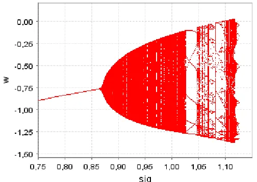
. Figure 3 presents a

bifurcation diagram for the first model (

ρ

=0). The Neimark-Sacker bifurcation is clearly

present, giving place to a region of a-periodic cycles and chaos.5

Note that, in our example,

θ

=1.149, and thus the bifurcation occurs at

87 . 0 149 . 1

1 =

=

σ

. To the left of this point, according to proposition 1 (and looking at

figure 3) stability prevails. The bifurcation diagram can, as well, be drawn for variable

vt (figure 4). We regard that cycles have a increasing amplitude and that there is the

possibility of this variable assuming negative values; this circumstance means that not

only all available credit is directed to consumption, but that also part of the current

resources available to invest in production are deviated to credit to consumption;

instability arises when the economic system becomes unable to sustain a situation where

a progressively larger amount of resources are allocated to finance future consumption.

The interpretation of figures 3 and 4 is essentially that if agents give little

importance to past deviations from the benchmark level of wealth (

σ

low), stability

holds. When this relevance rises, cycles set in and instability will end up by prevailing.

Bifurcation diagrams could be drawn as well for any other parameter, like the level of

financial development. We would have diagrams similar to the ones in the presented

figures, and the conclusion of the transition from stability to cycles and from these to

instability would be the same as the one depicted in the local analysis: instability (and,

before this state, a-periodic cycles) arise for a too high level of credit availability.

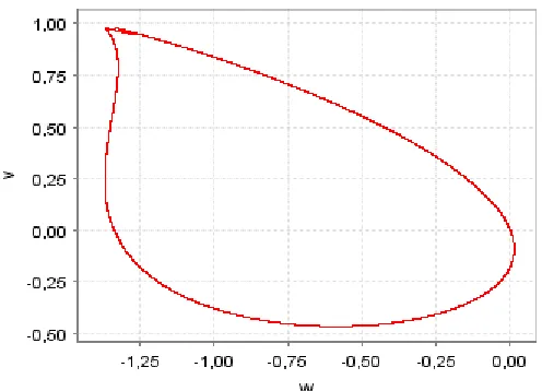
To illustrate further the cyclical nature of the results, we present through figures 5

and 6 the long term time series of wealth and an attracting set that defines the long run

relation between wt and vt; this is done for a value of

σ

for which chaotic behaviour is

evident.

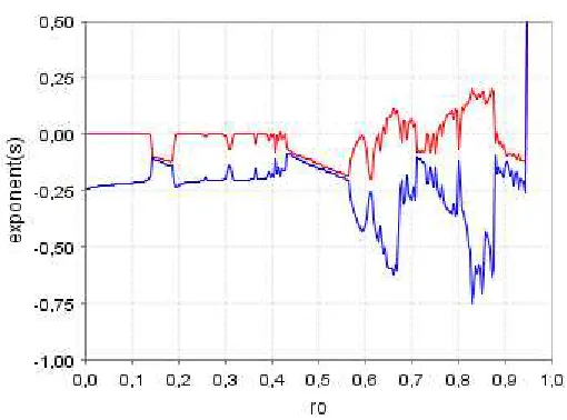
Finally, we can close the graphical analysis of this simplest case (

ρ

=0) with a

diagram that allows to identify rigorously the areas of chaotic motion. These are the

5

All the figures concerning global dynamics presented in this paper are drawn using IDMC software (interactive Dynamical Model Calculator). This is a free software program available at

ones for which at least one of the two Lyapunov characteristic exponents associated to

our system is positive. Recall that Lyapunov exponents are a measure of exponential

divergence of nearby orbits, that is, a measure of sensitive dependence on initial

conditions, which is a well accepted property of chaotic systems. See figure 7. Note, in

this figure, that for values of parameter

σ

around 0.85 to 1.03 one of the Lyapunov

exponents stays equal to zero; this is the result one expects to find in the presence of

quasi-periodic cycles, that is, cycles with no countable order but that are too regular to

be considered chaos (there is not an absolute dependence on initial conditions). Such a

result is the feature that commonly characterizes the state of a system immediately after

a Neimark-Sacker bifurcation. Chaotic motion is undoubtedly present for values of

σ

near 1.1.

To illustrate our second version of the model (

ρ

>0), we draw a diagram revealing

what kind of cycles one observes in the space of parameters (

σ

,

ρ

). We confirm the

analysis of section 3, in the sense that for relatively high values of

σ

, cycles arising from

a Neimark-Sacker bifurcation are identified, while relatively high values of

ρ

imply

cycles originating from a flip bifurcation (figure 8).

Let

σ

=1. For this value, figure 9 respects to a bifurcation diagram of the wealth

variable for different values of

ρ

, figures 10 and 11 draw time series and an attractor for

a specific value of

ρ

and figure 12 relates to Lyapunov exponents. Chaotic motion and

cycles of different periodicities are found for the wealth variable, and thus cyclical

motion will also be present in the time trajectories of other economic aggregates,

namely output, investment and consumption. Figure 11 reveals the higher sophistication

of the second considered case, in the sense that a ‘stranger’ (less regular) attractor is

obtained. Lyapunov exponents for different values of parameter

ρ

also show that

quasi-periodicity (one exponent equal to zero), periodic cycles and stability (both exponents

negative) and chaos (one positive exponent) coexist and alternate as we change the

value of the parameter.

The graphical analysis of this section was useful in characterizing the model

beyond local dynamics. The main new result is that an area of cycles and chaotic motion

is identified after the region of stability and before instability. Thus, for some

combinations of parameter values one is able to assert that the behaviour of economic

agents, in the case concerning credit decisions, can produce a situation of self sustained

cyclical motion, which is triggered by no monetary phenomena (Keynesian cycles) or

5. Final Remarks

We have developed a model of growth, cycles and financial development. A

standard growth model involving a constraint on credit was assumed, and over this

setup one has considered that part of the available credit is directed to productive

investment, while a second share is destined to anticipate in time households’

consumption. Under the assumption that the referred share varies with consumer

sentiment, and that this is influenced by contemporaneous and past economic

performance (more accurately, by the gap between effective and potential wealth in the

present and in the previous periods), we were able to furnish an explanation for

endogenous cycles.

Cycles of various periodicities and chaotic motion are observable for given

combinations of parameter values, and we found that the way wealth gaps impact over

credit allocation choices are one of the most relevant determinants of the stability results

(alongside with the level of financial development, the state of technology, the interest

rate, the savings rate and the economy’s growth rate). From a local analysis point of

view, one has concluded that both stability and instability can prevail, and that by

varying some parameters’ values a bifurcation (Neimark-Sacker or flip) is likely to

occur. When we search for the confirmation of these results through an analysis of

global dynamics, we are confronted with a region of cycles and chaos that follows the

point of bifurcation, before instability (divergence to zero or infinity) becomes

dominant.

From a policy point of view, the undertaken analysis is particularly important, in

the sense that it can give some hints on how to balance the allocation of credit to

consumption and to investment, in order to remain in the stability area, and therefore

avoid the welfare costs of cyclical motion.

References

Aghion, P.; P. Bacchetta and A. Banerjee (2004). “Financial Development and the

Instability of Open Economies.” Journal of Monetary Economics, vol. 51, pp.

1077-1106.

Aghion, P.; A. Banerjee and T. Piketty (1999). “Dualism and Macroeconomic

Aloi, M.; H. D. Dixon and T. Lloyd-Braga (2000). “Endogenous Fluctuations in an

Open Economy with Increasing Returns to Scale”, Journal of Economic Dynamics

and Control, vol. 24, pp. 97-125.

Amable, B.; J. B. Chatelain and K. Ralf (2004). “Credit Rationing, Profit Accumulation

and Economic Growth.” Economics Letters, vol. 85, pp. 301-307.

Benhabib, J. and R. H. Day (1981). “Rational Choice and Erratic Behaviour.” Review of

Economic Studies, vol. 48, pp. 459-471.

Bernanke, B. and M. Gertler (1989). “Agency Costs, Net Worth, and Business

Fluctuations.” American Economic Review, vol. 79, pp. 14-31.

Boldrin, M. and L. Montrucchio (1986). “On the Indeterminacy of Capital

Accumulation Paths.” Journal of Economic Theory, vol. 40, pp. 26-39.

Boldrin, M.; K. Nishimura; T. Shigoka and M. Yano (2001). “Chaotic Equilibrium

Dynamics in Endogenous Growth Models.” Journal of Economic Theory, vol. 96,

pp. 97-132.

Caballé, J.; X. Jarque and E. Michetti (2006). “Chaotic Dynamics in Credit Constrained

Emerging Economies.” Journal of Economic Dynamics and Control, vol. 30, pp.

1261-1275.

Cazavillan, G.; T. Lloyd-Braga and P. Pintus (1998). “Multiple Steady-States and

Endogenous Fluctuations with Increasing Returns to Scale in Production.” Journal

of Economic Theory, vol. 80, pp. 60-107.

Cellarier, L. (2006). “Constant Gain Learning and Business Cycles.” Journal of

Macroeconomics, vol. 28, pp. 51-85.

Christiano, L. and S. Harrison (1999). “Chaos, Sunspots and Automatic Stabilizers.”

Journal of Monetary Economics, vol. 44, pp. 3-31.

Day, R. H. (1982). “Irregular Growth Cycles.” American Economic Review, vol. 72,

pp.406-414.

Deneckere, R. and S. Pelikan (1986). “Competitive Chaos.” Journal of Economic

Theory, vol. 40, pp. 13-25.

Gomes, O. (2006). “Routes to Chaos in Macroeconomic Theory.” Journal of Economic

Studies, vol. 33, pp. 437-468.

Grandmont, J. M. (1985). “On Endogenous Competitive Business Cycles.”

Econometrica, vol. 53, pp. 995-1045.

Guo, J. T. and K. J. Lansing (2002). “Fiscal Policy, Increasing Returns and Endogenous

Kyotaki, N. and J. Moore (1997). “Credit Cycles.” Journal of Political Economy, vol.

105, pp. 211-248.

Levine, R. (1997). “Financial Development and Economic Growth: Views and

Agenda.” Journal of Economic Literature, vol. 35, pp. 688-726.

Levine, R. (2005). “Finance and Growth: Theory and Evidence.” in P. Aghion and S. N.

Durlauf (eds.), Handbook of Economic Growth, Amsterdam: Elsevier, pp.

865-934.

Lloyd-Braga, T.; C. Nourry and A. Venditti (2006). “Indeterminacy in Dynamic

Models: When Diamond Meets Ramsey.” Journal of Economic Theory,

forthcoming.

Mitra, T.; K. Nishimura and G. Sorger (2005). “Optimal Cycles and Chaos.” Cornell

University, Kyoto University and University of Vienna working paper.

Schmitt-Grohé, S. (2000). “Endogenous Business Cycles and the Dynamics of Output,

[image:17.595.110.479.127.750.2]

Figures

[image:17.595.176.428.560.739.2]

Figure 1 – Local dynamics; ρρρρ=0.

Figure 2 – Local dynamics; ρρρρ>0.

Figure 3 – Bifurcation diagram (w~_t;σσσσ);ρρρρ=0.

Tr(J) 1

Det(J)=1 Det(J)

1+Tr(J)+Det(J)=0 1-Tr(J)+Det(J)=0 Tr(J) 1

Det(J)=1 Det(J)

[image:18.595.178.427.79.260.2] [image:18.595.172.426.314.496.2]

Figure 4 – Bifurcation diagram (vt;σσσσ);ρρρρ=0.

Figure 5 – Long run time series of w~_t; σσσσ=1.11, ρρρρ=0.

Figure 6 – Attractor (w~_t;vt) ; σσσσ=1.11, ρρρρ=0

[image:18.595.178.426.551.730.2]

[image:19.595.176.425.78.263.2] [image:19.595.175.425.315.502.2]

Figure 7 – Lyapunov characteristic exponents;ρρρρ=0.

Figure 8 – Cycles in the space of parameters; ρρρρ>0.

[image:19.595.179.428.562.745.2]

[image:20.595.179.426.79.260.2] [image:20.595.178.429.314.496.2]

Figure 10 – Long run time trajectory of w~_t; σσσσ=1, ρρρρ=0.85.

Figure 11 – Attractor (w~_t;vt) ; σσσσ=1, ρρρρ=0.85

(the first 10.000 observations are excluded).

[image:20.595.175.430.560.749.2]