EOQ Model with Partial Backordering for Imperfect Items
under the Effect of Inflation and Learning with Selling
Price Dependent Demand
Dharmendra Yadav
Department of Mathematics Vardhaman (P.G) College
Bijnor-246701 (U.P) India
S.R. Singh
Department of Mathematics D.N. (P.G) College, Meerut-250001(U.P) India
Meenu
Department of Mathematics Banasthali University Banasthali-304022 (Rajasthan)
India
ABSTRACT
One of the most fruitful areas in the line of inventory is that the deficiency of handling/ production facilities can be overcome through a natural phenomenon known as learning effect. Due to this the performance of service and manufacturing organizations engaged in a repetitive process improves with time. The proposed economic order quantity model (EOQ) in this paper has been made realistic by analyzing the impact of learning. All of the study is carried out in inflationary environment. It is very obvious fact that given some time, every item can create a niche for itself in the customer’s mind, hence increasing its demand with the passage of time. The selling price of a product is one of the crucial factors in selecting the item for use. Keeping this in mind, an inventory model is developed by taking selling price dependent demand. In this model, it is assumed that the received items are not of perfect quality and after100% screening, imperfect items are withdrawn from inventory and sold at discounted price. Finally, the feasibility and applicability of model are shown through numerical analysis. Sensitivity analysis is also performed with respect to different inventory parameters.
Keywords
EOQ, Partial Backordering, Imperfect Items, Inflation, Learning, Selling Price Dependent Demand
1.
INTRODUCTION
Nowadays, inventory management becomes a passion of decision-makers. The Decision-makers left no stone unturned while making inventory policy to get the competitive advantages. In this direction, one of the most fruitful areas in the line of inventory management is that the deficiency of manufacturing/handling facilities can be overcome through a natural phenomenon known as learning effect. Due to this the capacity of manufacturing and service organizations engaged in a repetitive process improves with time.
In the past, many inventory practitioners while making inventory policy assumed that 100% of perfect quality items are present in each ordered items. But, in real life situation it is not so. Presence of imperfect items in ordered lot is due to natural disasters, damage or breakage in transit and many more reasons. Therefore, the lot manufactured/ received may contains some defective items. Nowadays, there is a trend to develop inventory policy for real life situations. So, while developing an inventory control policy, one should develop model with this assumption that each lot not contains 100% perfect items. In the model developed by Rosenblatt and Lee’s (1986), it was found that they assumed that the defective items could be reworked instantaneously at a cost and the presence of defective products motivates decision
maker to order smaller lot sizes. They assumed that the time between the in-control state and the out-of-control state is exponential distributed. Kim and Hong (1999) extended the model of Rosenblatt and Lee by using the distribution of the time between the in-control state and the out-control state.
Salameh and Jaber (2000) assumed that the imperfect items present in each lot not necessary defective items could be sold as a single batch at a discounted price prior to receiving the next shipment. They observed that the economic lot size quantity tends to increase as the average percentage of imperfect quality items decreases. After that several researchers extended the work of Salameh and Jaber (2000)
in different direction. Goyal and Cádenas-Barrόn (2002)
reconsidered the model formulated by Salameh and Jaber (2000) and presented a simple approach for determining the optimal lot size. Chang (2004) determined the optimal order lot size to maximize the total profit when lot contains imperfect quality items. Huang (2004) extended Salameh and Jaber’s (2000) work in the integrated production and shipping context while Papachristos and Konstantaras (2006) proposed sufficient conditions for the model proposed by Salameh and Jaber’s (2000).Maddah and Jaber (2008)
modified the model of Salameh and Jaber (2000) by applying renewal theory to obtain the expected profit per unit time. Roy et al. (2011) developed an economic order quantity model in which a certain items of ordered quantity are of imperfect quality. Yadav et al. (2012) developed an inventory model to deal the fuzziness aspect of demand and effect of learning on holding cost, ordering cost and number of defective items present in each lot. In this model, they assumed that the received items are not of perfect quality and after100% screening, imperfect items are withdrawn from inventory and sold at discounted price. Yadav et al. (2012)
incorporated the effect of learning in holding cost, ordering cost and on the number of defective items present in each lot. They used algebraic method to determine the optimal values.
Goyal et al. (2015) investigated an Economic Order Quantity model in which the demand of items is fuzzy in nature and depends on the advertisement frequency. They formulated model by incorporate learning effects on number of defective items present in each lot and the possibility of lost sale and backorder.
the quality of the product improves in each lot because of learning; this is due to the familiarity with the set-up, the tooling, instructions, blueprints, the workplace arrangement, and the condition of the process.
It was very obvious fact that given some time, every item can create a niche for itself in the customer’s mind, hence increasing its demand with the passage of time. In the present market, the selling price of a product is one of the crucial factors in selecting the item for use. In practice, lower selling price of a product increases the demand where as high price has a reverse effect. Very few inventory practitioners and researchers studied the effects of selling price on demand. First time, Whitin (1955) presented an inventory model considering the effect of price dependent demand. Generally this type of demand is seen in finished goods. Burwell et al. (1997) developed an economic lot size model for price dependent demand under quantity and freight discounts.
Mondal et al. (2003) presented an inventory system of ameliorating items for price dependent demand rate. You (2005) developed an inventory model with price and time dependent demand. Teng et al. (2005) developed an inventory model with price dependent demand rate. In 2009, Maiti et al.
developed an inventory model for an item in stochastic environment with price-dependent demand over a finite time horizon. Chang et al. (2010) developed the inventory model with the problem of determining the optimal selling price and order quantity simultaneously under EOQ model for deteriorating items. It is assumed that the demand rate depends not only on the on-display stock level but also the selling price per unit, as well as the amount of shelf/display space is limited. Shastri et al. (2014) developed a supply chain inventory model for deteriorating items to determine the optimal ordering policies of a retailer under two levels of trade credit to reflect the SCM situation has been developed. Further, they assumed that demand rate of the product is the function of selling price.
Buzacott (1975) was the first who developed an inventory model by assuming a constant inflation rate. Misra (1979)
developed an inflation model for the economic order quantity model, by considering the time value of money and different inflation rates. Liao et al. (2000) investigated the effect of inflation on a deteriorating inventory when supplier permitted delay in payment. Yang (2004) proposed an inventory model for deteriorating items stored at two warehouses when inflation is prevalent. Chern et al. (2008) extended the traditional inventory lot-size model to allow for general partial backlogging rate and inflation. Min et al. (2012) investigated an inventory model for exponentially deteriorating items under the conditions of permissible delay in payments. Yadav et al. (2015) developed the retailer’s inventory model to
determine the optimal cycle time and payment time of the retailer in an inflationary environment. They assumed that the retailer can pay the supplier either at the end of the credit period or later pay interest on the unpaid amount for the overdue period.
It is observed that, most of the inventory practitioners in their work assumed that there is no shortages during planning horizon and very few of them considered that demand during stock out period is either completely backordered or lost. However, this seems to be unrealistic as a fraction of customers are always willing to wait for their order to be fulfilled by the retailer whereas others switch over to somewhere else. Therefore, for inventory models where shortages are allowed, it is more reasonable to assume that some of the excess demand is backordered and rest of will
lost. It is observed that Salameh and Jaber (2000), Chang (2004), Huang (2004), Papachiristos and Konstantaras (2006), Jaber et al. (2008) all discussed imperfect items present in lot but no one considered shortages. Kim and Park (1985) investigated an inventory model with a mixture of sales and time weighted backordered. Pan and Hsiao (2005)
presented inventory model with backordered. Yadav et al. (2012) developed an economic order quantity model by incorporating the effect of learning in holding cost, ordering cost and on the number of defective items present in each lot. They also considered that shortage quantities will backordered. Over production or over carrying is not a solution due to higher carrying cost of the product. Due to presence of imperfect items in each lot, shortages cannot be ignored while developing inventory model. It seems to be more reasonable to assume that only fraction of customers are ready to wait during stock out period for their delivery while rest of go to other place. Therefore, taking all of this in account, it is considered that that shortage during stock out period is partially backordered.
The present paper analyzes the impact of learning on optimal solution of inventory problem. All of the study is carried out in inflationary environment. In this paper an inventory model is developed by taking selling price dependent demand. Effect of learning on number of imperfect items present in each lot is also considered. In this model, it is assumed that the received items are not of perfect quality and after100% screening, imperfect items are withdrawn from inventory and sold at discounted price. Concepts of learning by doing are best fitted in industry such as automotive and stabilizer industry. In these industries, number of imperfect items reduces from one shipment to another due to learning effect. Finally, the feasibility and applicability of model are shown through numerical analysis. Sensitivity analysis is also carried out with respect to different inventory parameters.
2.
ASSUMPTIONS AND NOTATIONS
Assumptions
In this paper, mathematical model is developed under the following assumptions.
1. Single type of items is involved in the inventory system.
2. The replenishment rate is infinite.
3. Demand rate consider as the function of selling price.
4. The screening process and demand proceed simultaneously. But it is assumed that the screening rate is greater than demand rate, i.e., x>D(s)
5. Each lot contains defective items. The number of defective items present in each lot follows a learning curve.
6. After the completion of the screening process, the defective items are sold at a discounted price in a single batch.
7. Inflation and time value of money is considered.
8. Lead-time is negligible.
9. Shortages are allowed and partially backlogged.
10. Demand of the customers is satisfied by good quality items only.
Notations:
Following notations are used for the development of mathematical model in this section:
: Demand rate measured in units per unit of time
Which depends on selling price
k : Constant representing the difference between discount rate (k1) and inflation rate (k2).
yn : Order quantity in units for the n th
shipment, where
n
1c(t) : Unit purchasing cost per item at time t, i.e., C(t) = , where c is the purchasing cost at time
zero
K(t) : Unit ordering cost per item at time t, i.e., K(t) =K , where K is the ordering cost at time zero
h(t) : Unit holding cost per item at time t, i.e., h(t) =h , where h is the holding cost at time zero
s(t) : Unit selling price per item at time t, i.e., s(t) =s , where s is the selling price at time zero
cl(t) : Unit lost sale cost per item at time t, i.e., cl(t)
= , where is the lost sale cost at time zero
cb(t) : Unit backordering cost per item at time t, i.e.,
cb(t) = , where is the backordering cost
at time zero
v(t) : Unit discount price per item at time t, i.e., v(t) = , where is the discount price at time
zero, v<c
Sc(t) : Unit screening cost per item at time t, i.e., Sc(t)
= , where is the sreening cost at time
zero
p(n) : Percentage of defective items in each shipment
follows the learning curve
bn
a g e
,
a,b,g>0
Tn : Cycle time per shipment
x : Screening rate measured in units per unit of time t1n : Time to screen yn units, where t1n=yn/x<Tn
B : Maximum backordering quantity in units
: Rate of partial backordering
T1n : Time where inventory level reaches to zero
3.
THE MATHEMATICAL MODEL
It is assumed that yn items are procured at the beginning of
each cycle. This quantity is used to satisfy the demand during positive inventory level and backordering quantity during shortages. Each lot contains good as well as poor defective items. Inspection process starts at the rate ‘x’ from the beginning of each cycle. It is assumed that the rate of inspection is more than the demand rate. tn is the time when
the screening process is completed. During the screening process, the demand of the items occurs parallel to the screening process. During this period, demand satisfied from the items which are found to be of perfect quality by the screening process. At that moment, items of poor quality are sorted, kept in stock and sold at a salvage value at a
discounted price. To avoid the shortages of good items within the screening time t1n(=yn/x), p(n) must satisfies the following
restriction:
i.e., …. (1)
Mathematically, inventory level at any time t during the positive inventory level can be represented by the following differential equation:
…. (2)
On solving the above differential equation using the boundary condition (0)=yn- , we get
…. (3)
Inventory level at any time t1n is
…. (4)
Number of defective items = p(n)yn
Therefore, the inventory level of good items during t1n≤t≤
is
…. (5)
We have which gives
…. (6)
Mathematically, inventory level during shortage period can be represented by the following differential equation:
…. (7)
On solving the above differential equation by using the boundary condition ( )=0, we get inventory level at
time ‘t’ is
…. (8) Inventory level at time Tn is , therefore we get
…. (9)
From equation (6) and (9), we get
…. (10)
Now, we can evaluate different cost which is associated inventory step by step.
Holding cost =
Ordering cost = K(0)+ K(T)+ K(2T)+………+ K((m-1)T)+………
Purchase cost = c(0) yn+ c(T) yn+ c(2T) yn+………+
c((m-1)T) yn+………
Screening cost = Sc(0)yn+ Sc(T)yn+ Sc(2T)yn+…+ Sc ((m-1)T)
yn+……..
Selling price of good items = (s(0) + s(T) + s(2T) +….+ s ((m-1)T) +…) yn(1-p(n)
Selling price of defective items = (v(0) + v(T) + v(2T) +….+ v ((m-1)T) +…) ynp(n)
Backlogging cost =
Lost sale cost =
=
The total revenue per cycle, TR(yn), is the sum of total sales
volume of good quality and imperfect quality items.
Therefore, TR(yn)
…. (11)
The total cost per cycle TC(yn) is the sum of ordering cost,
purchasing cost, screening cost and holding cost. TC(yn)=
…. (12)
Total profit of the retailer is TP= TR(yn)- TC(yn)
or
…. (13)
Our objective is to find the value of yn and Tn in order that the
profit of the retailer is maximum.
For this, we set
…. (14)
…. (15)
From equation (14), we get
…. (16) On putting the value of from equation (16) in equation (15), we get the value of and hence from equation (14) we get
4.
NUMERICAL ANALYSIS
In order to illustrate the results of the proposed models, an inventory system with screening cost Sc=$0.5/unit, purchase cost c=$25/unit, selling price of good-quality items s=$50/unit, selling price of imperfect-quality items v=$20/unit, ordering cost K=$100/cycle, holding cost h=$10/unit/year is considered. It is assumed that the number of defective items present in each lot is deterministic in nature and follows a learning curve. The values of the other parameters are as follows:
e=40, f=999, d=50,000 units/year, screening rate x= 175200 units/year, n=1
Using the above mentioned values and Microsoft Excel Solver, we get the optimal values of decision variables which are as follows:
yn=1750 unit, Tn=0.78 and Profit =$9048949
5.
SENSITIVITY ANALYSES
The change in the value of parameters may happen due to uncertainties in any decision-making situation. In order to examine the implication of these changes, the sensitivity analysis is of great help in decision-making. Using the data given in the nemerical section, the sensitivity analysis with respect to different parameters are carried out here.
5.1
Sensitivity Analysis with respect to
selling price
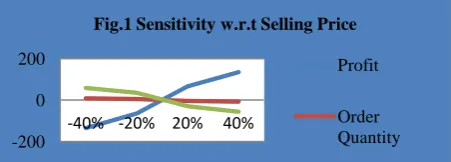
From Fig.1 it is observed that optimal decision is highly sensitive with respect to selling price. As the selling price of the perfect items increases total profit of the system increases whereas the ordering quantity and the replenishment time decreases. As the selling price increases the demand of the items decreases and hence ordering quantity and the replenishment time decreases.
5.2
Sensitivity Analysis with respect to
selling price of Imperfect Items
To discuss the effect of selling price of imperfect items on the optimal values of decision variable we change it from -40% to 40%. Its effect is represented in Fig.2.
From Fig.2 it is observed that optimal decision is not sensitive with respect to selling price. There is very little fluctuation in the optimal decision with respect to the change in selling price of imperfect items.
5.3 Sensitivity Analysis with respect to
Demand
We know that demand play an important role while taking the decision regarding inventory. So it is important to analyze the sensitivity with respect to demand. Its effect on optimal values is represented in Fig.3.
From the Fig.3 it is observed that as the demand of the items increases the profit of the system increases and to meet out the increase in demand the ordering quantity and hence replenishment time increases. Thus demand has the positive impact on the decision variables.
5.4 Sensitivity Analysis with respect to
holding Cost
Holding cost has adverse effect on the optimal solution. To analyze the effect of holding on the optimal values of the decision variables the sensitivity analysis is performed here with respect to the holding cost. It is represented in Fig.4.
From Fig.4 it is observed that holding cost has significant effect on the optimal values of decision variables. As the holding cost decreases decision makers always try to stock more inventory so the ordering quantity increases and hence replenishment time also increases. Holding cost has very little effect on the profit of the system.
5.5 Sensitivity Analysis with respect to
Inflation
Inflation is the state of a continuous increase in price of goods and service. Hence, as obvious, rate of inflation causes changes in the optimal decision. So it is interesting to carry out the sensitivity with respect to inflation. It is shown with help of Fig.5.
An increase in the rate of inflation causes the total profit of the system going down. Such a change in the system is very appreciable. An increase in the inflation rate reduces the purchasing power. So decision-maker can buy fewer inventories, which ultimately finish off sooner.
5.6 Sensitivity Analysis with respect to
Backlogging Rate
In order to study the effect of backlogging rate on optimal solution of the proposed inventory model, a sensitive analysis with respect to it is performed here. Variation in backlogging rate from -40% to 40% is considered and the effect on optimal solution is presented Fig.6.
Fig.6 represents the effects of backlogging fraction on the optimal solution. As the value of δ increases, total ordering quantity and replenishment time increases while the total profit decreases due increase in the backordering cost. So, planned partial backordering is advisable in place of full backorder or lost sale.
5.7 Sensitivity Analysis with respect to
Screening Rate
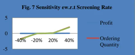
Sensitive analysis is performed with respect to screening rate to analyze its influence on optimal solution. It is represented in Fig.7.
-200 0 200
[image:5.595.56.282.73.154.2]-40% -20% 20% 40%
Fig.1 Sensitivity w.r.t Selling Price
Profit
Order Quantity
-10 0 10
[image:5.595.316.541.74.154.2]-40% -20% 20% 40%
Fig.2 Sensitivity Analysis w.r.t Selling Price of Imperfect Items
Profit
Order Quantity
-200 0 200
[image:5.595.57.278.296.390.2]-40% -20% 20% 40%
Fig. 3 Sensitivity w.r.t Demand
Profit
Ordering Quantity
-50 0 50
-40% -20% 20% 40%
Fig.4 Sensitivity w.r.t Holding Cost
Profit
Ordering Quantity
-40 -20 0 20 40
[image:5.595.317.542.313.403.2]-40% -20% 20% 40%
Fig. 5 Sensitivity w.r.t Inflation
Profit
Ordering Quantity
-100 0 100
[image:5.595.55.284.519.603.2]-40% -20% 20% 40%
Fig. 6 Sensitivity w.r.t Backlogging Rate
Profit
[image:5.595.317.541.559.632.2]From Fig.7 it is observed that as the screening rate increases the profit of the system also increases due to the lower inventory cost. As a result, the ordering cost and the replenishment cost increases. It is observed that screening rate has less effect on the optimal solution on compared to the other parameters.
5.8 Effect of Learning on optimal solution
Now, we analyze the effect of learning of the number of imperfect items present in each lot and the profit of the system.Fig.8 reflects that when there is effect of learning on number of imperfect items present in each lot then ordering quantity decreases in each cycle. In this scenario managers should order smaller lots so that by learning, the number of imperfect items decreases in each lot and they can earn more profit for the organization.
6.
SUMMARY AND CONCLUDING
REMARKS
Due to stiff competition in the market, customers have lot of choices and there is little to stop them from going to the next shop if the current service provider can’t satisfy them. So, inventory practitioner concentrates himself to explore the opportunities in all directions in order to increase customer’s service and his profit. So while developing the inventory policy, inventory practitioner may consider learning effect, partial backordering and effect of inflation to reduce inventory cost and improve profitability of the business. Model developed in this paper can be used in chemical, food, nuclear and stabilizer industries.
This paper extends economic order quantity model to explicitly specify the effects of learning phenomenon on number of imperfect items present in each lot and partial backlogging in inflationary environment.
The result shows that number of imperfect units and the ordering quantity decreases whereas net profit increases as learning increases following a form of the logistic curve. As learning becomes faster it is suggested to order in smaller lots less frequently. Thus a manager should keep his learning process in all directions to earn more profit for the organization. Numerical example shows that partial backlogging is better than the total backordering.
On summing it can say that this model provide a remedy for the quick changes in the market performance of any product and hence, can act as a savior for the inventory practitioner by
offering him quick remedies. Model presented in this paper, have been tested numerically and have also been proved financially viable too.
In future research the impact of stochastic learning curve on the above models can be discussed. This model can be extended by considering n equal cycles for finite time horizon.
7.
REFERENCES
[1] Burwell T. H., Dave D. S., Fitzpatrick K. E. and Roy M. R. (1997). Economic lot size model for price-dependent demand under quantity and freight discounts, International Journal of Production Economics, Vol. 48(2), pp.141-155.
[2] Buzacott, J.A. (1975). Economic order quantities with inflation. Operational Research Quarterly, Vol. 26, pp. 553-558.
[3] Chang, C.T., Chen, Y.J., Tsai, T.R., and Wu, S.J. (2010). Inventory models with stock-and price dependent demand for deteriorating items based on limited shelf space. Yugoslav Journal of Operations Research, Vol. 20(1), pp.55-69.
[4] Chang, H.C. (2004). An application of fuzzy sets theory to the EOQ model with imperfect quality items. Computers and Operational Research, Vol. 31, pp. 2079-2092.
[5] Chern, M.S., Yang, H.L., Teng, J.T., and Papachristos, S. (2008). Partial backlogging inventory lot-size models for deteriorating items with fluctuating demand under inflation. European Journal of Operational Research, Vol.191 (1), pp.127-141.
[6] Goyal, S.K., and Cardenas-Barron, L.E. (2002). Note on economic production quality model for items with imperfect quality-A practical Approach. International Journal of Production Economics, Vol. 77, pp. 85-87.
[7] Goyal, S.K., Singh, S.R., and Yadav, D. (2015). A New Approach for EOQ Model for Imperfect Lot Size with Mixture of Backorder and Lost Sale under Advertisement Dependent Imprecise Demand. International Journal of Operational Research, (accepted).
[8] Huang, C.K. (2004). An optimal policy for a single-vendor single-buyer integrated production-inventory problem with process unreliability. International Journal of Production Economics, Vol.91, pp. 91-98.
[9] Jaber, M.Y., Goyal, S.K., and Imran, M. (2008). Economic production quantity model for items with imperfect quality subject to learning effects. International Journal of Production Economics, Vol.115, pp.143-150.
[10]Kim, C.H., and Hong, Y. (1999). An optimal production run length in deteriorating production process. International Journal of Production Economics, Vol. 58, pp. 183-189.
[11]Kim, D.H., and Park, K.S. (1985). (Q, r) inventory model with a mixture of sales and time weighted backorders. Journal of the Operational Research Society, Vol.36, pp.231-238.
[12]Liao, H.C., Tsai, C.H., and Su, C.T. (2000). An inventory model with deteriorating items under inflation when a delay in payment is permissible. International Journal of Production Economics, Vol.63, pp. 207-214.
-5 0 5
[image:6.595.57.278.73.164.2]-40% -20% 20% 40%
Fig. 7 Sensitivity ew.r.t Screening Rate
Profit
Ordering Quantity
-50 0 50
[image:6.595.55.279.292.372.2]-40% -20% 20% 40%
Fig. 8 Effect of Learning of Decision Variables
[13]Maddah, B., and Jaber, M.Y. (2008). Economic order quantity for items imperfect quality: Revisited. International Journal of Production Economics, Vol.112, pp.808-815.
[14]Maiti, A., Mait, M., and Maiti, M. (2009). Inventory model with stochastic lead-time and price dependent demand in corporating advance payment. Applied Mathematical Modelling, Vol. 33(5), pp. 2433-2443.
[15]Min, J., Zhou, Y.W., Liu, G.Q., and Wang, S.D. (2012). An EPQ Model for Deteriorating Items with Inventory-Level-Dependent Demand and Permissible Delay in Payments. International Journal of Systems Science, Vol. 43(6), pp.1039-1053.
[16]Misra, R.B. (1975). A study of inflationary effects on inventory systems. Logistic Spectrum, Vol. 9(3), pp.260-268.
[17]Mondal B., Bhunia A. K. and Maiti M. (2003). An inventory system of ameliorating items for price dependent demand rate, Computers and Industrial Engineering, Vol. 45(3), pp. 443-456.
[18]Pan, C.H., and Hsiao, Y.C. (2005). Integrated inventory models with controllable lead time and backorder discount considerations. International Journal of Production Economics, Vol.93, pp.387-397.
[19]Papachristos, S., and Konstantaras, I. (2006). Economic ordering quantity models for items with imperfect quality. International Journal of Production Economics, Vol.100, pp.148-154.
[20]Rosenblatt, M.J., and Lee, H.L. (1986). Economic production cycles with imperfect production process. IEE Transactions, Vol. 18, pp. 48-55.
[21]Roy. M.D., Sana, S.S., and Chaudhuri, K.S. (2011). An economic order quantity model of imperfect quality
items with partial backlogging. International Journal of Systems Science, Vol. 42(8), pp. 1409-1419.
[22]Salameh, M.K., and Jaber, M.Y. (2000). Economic production quantity model for item of imperfect quality. International Journal of Production Economics, Vol. 64, pp.59-64.
[23] Shastri, A., Singh, S.R., Yadav, D., and Gupta, S. (2014). Supply chain management for two-level trade credit financing with selling price dependent demand under the effect of preservation technology. Int. J. of Procurement Management, Vol. 7(6), pp.695-718.
[24]Teng, J. T., Chang, C. T., and Goyal, S. K. (2005). Optimal pricing and ordering policy under permissible delay in payments, International Journal of Production Economics, Vol. 97, pp.121-129.
[25]Whitin, T. M. (1955). Inventory control and price theory. Management Sci., Vol. 2, pp. 61–80.
[26]Yadav, D., Singh, S.R., and Kumari, R. (2012). Effect of Demand Boosting Policy on Optimal Inventory Policy for Imperfect Lot Size and with Backorder in Fuzzy Environment. Control and Cybernetics, Vol. 43(1), pp.191-212.
[27]Yadav, D., Singh, S.R., and Kumari, R. (2012). Effects of Learning on Optimal Lot Size and Profit in Fuzzy Environment. International Journal of Operational and Quantitative Management, Vol. 18(2), pp.145-158.
[28]Yadav, D., Singh, S.R., and Kumari, R. (2015). Retailer’s optimal policy under inflation in fuzzy environment with trade credit. International Journal of Systems Science, Vol. 46(4), pp. 754-762.