http://dx.doi.org/10.4236/ojepi.2016.61007
How to cite this paper: Karam, H.A., da Silva, J.C.B., Filho, A.J.P. and Rojas, J.L.F. (2016) Dynamic Modelling of Dengue Epi-demics in Function of Available Enthalpy and Rainfall. Open Journal of Epidemiology, 6, 50-79.
http://dx.doi.org/10.4236/ojepi.2016.61007
Dynamic Modelling of Dengue Epidemics in
Function of Available Enthalpy and Rainfall
Hugo Abi Karam
1*, Julio Cesar Barreto da Silva
2, Augusto José Pereira Filho
3,
José Luis Flores Rojas
31Instituto de Geociências, IGEO-CCMN-UFRJ, Universidade Federal do Rio de Janeiro, Rio de Janeiro, Brasil 2Departmento de Estatística, CCET-UFRN, Universidade Federal do Rio Grande do Norte, Natal, Brasil 3Instituto de Astronomia, Geofísica e Ciências Atmosféricas, IAG-USP, Universidade de São Paulo, SP, Brasil
Received 1 December 2015; accepted 20 February 2016; published 23 February 2016
Copyright © 2016 by authors and Scientific Research Publishing Inc.
This work is licensed under the Creative Commons Attribution International License (CC BY). http://creativecommons.org/licenses/by/4.0/
Abstract
In this work, we present results of an investigation of environmental precursors of infectious epi-demic of dengue fever in the Metropolitan Area of Rio de Janeiro, RJ, Brazil, obtained by a numeri-cal model with representation of infection and reinfection of the population. The period consi-dered extend between 2000 and 2011, in which it was possible to pair meteorological data and the reporting of dengue patients worsening. These data should also be considered in the numerical model, by assimilation, to obtain simulations of Dengue epidemics. The model contains compart-ments for the human population, for the vector Aedes aegypti and four virus serotypes. The results provide consistent evidence that worsening infection and disease outbreaks are due to the occur-rence of environmental precursors, as the dynamics of the accumulation of water in the breeding and energy availability in the form of metabolic activation enthalpy during pre-epidemic periods.
Keywords
Modelling Dengue Epidemics, Environmental Enthalpy, Environmental Precursors of Dengue Epidemics
1. Introduction
Dengue fever is an acute viral disease of fast dissemination, featured by an infirmity that is caused by the Dengue fever virus, an arbovirus of the family Flaviviridae, genus Flavivirus, which comprises 4 immunological types (i.e. serotypes) which are activelly circulating among humans (DENV-1, DENV-2, DENV-3 and DENV-4)
[1]. Surprisiling, a new type (DENV-5) was identified by Nikos Vasilakis in 2013 [2]. Nowadays, Dengue fever epidemics is a serious public health global issue [1].
In Brazil, Dengue fever infections have been reported since 1986 [3], but only after 2015, the 4 serotypes have been found in Brazil [4]-[6].
The primary infection caused by any one of the serotypes can provide permanent protection against reinfec- tion by the same serotype and temporary protection against the remaining serotype [7]. In general, the natural growth of population exposes a new group of humans to primary infection of the viruses [8].
According to the 2005 technical relatory from the Brazilian Wealth Surveilance Service (Serviço de Vigilân- cia em Saúde) [9], the epidemic situation was of the most severe among countries of tropics, in highly urbanized regions where the Aedes aegypti, the mosquito vector of Dengue fever, can easily breed.
The viremia period on humans is of seven days, being shorter on other primates [10]. The Dengue may occur as Dengue Fever, the most benign and frequent form of Dengue, but it can also occur as Dengue Haemorrhagic Fever, a much more severe manifestation, causing death in approximately 5% of the reinfected patients [11].
The Dengue vector is the Aedes aegypti mosquito that has two distinct phases in its life cycle: aquatic, which comprehends the stages of egg, larva and pupa; and winged, also known as adult phase [12]. In each of those phases and stages specific mortality occurs. There are also distinct transition times from a stage to another.
When the mosquito transmits the disease to a human, through the inoculation of the virus, an incubation period called viremia starts in the human organism. After the contamination, the virus remains in the human blood from the day before the fever to the sixth day of disease. In this period, a non-infected female Aedes aegypti that bites the infected human, also contaminates itself, initiating the extrinsic incubation process [10]. The Dengue virus is not harmful to the mosquito, and once infected it becomes a permanent vector.
The life cycle of the Dengue vector is well known. For a extensive description see Christophers (1960) [12]. A simple description was given by the researchers of Fundação Oswaldo Cruz (FIOCRUZ) in Rio de Janeiro-RJ [13] [14].
In a summarized form, only the virus infected female Aedes aegypti mosquitoes are able to transmit the disease to men. The specificity of females as a vector of the virus is due to the haematophagous nutrition necessary to mature the eggs [12]. The regular nutrition of male and female Aedes aegypti is based on liquids containing sugars and sap from plants. The virus presence in the salivary glands of the vector occurs after the extrinsic incubation period, which lasts from the blood ingestion to the moment in which the mosquito will be able to transmit the virus, which will be largely replicated in its salivary glands and nervous system. This period varies from 8 to 14 days, from the moment the female mosquito bites an infected human, takes the human blood and receives the virus that goes to its pharynx. The virus then is absorbed and spread to the insect organism until the virus is concentrated in the salivary glands and brain of the mosquito. Then the virus replicates, enabling the inoculation on a human. In high temperatures this incubation period can be shortened in three days. In some cases the virus may replicate in the ovary and other reproductive system tissues of the mosquito. When this happens part of the female mosquito cubs are born with the virus, which can be transmitted by hereditary. Because of this Aedes aegypti mosquitoes may be flying around infected without register of human infections [13] [14].
According to Brigdman and Oliver (2006) [15], projections from the first half of the XXI century suggest a mean urban population growth of 2% per year; thus in 2050 it is estimated that 65% of the world population will live in cities, with incresing higher temperatures, associated with the global warming and also the development of Urban Heat Islands (UHI).
In the present work, a numerical model was proposed in the form of a set of coupled non-linear partial differential equations used to simulate the epidemic dynamics in the human population, vectors and virus. The model equations were designed to permit representation of Dengue fever infections, as also the assimilation of atmospheric observed data, including air temperature, pressure, umidade, precipitation, shortwave irradiance, etc. The simulated period was between Jan./2000 and Dec./2011, when Dengue fever epidemics were observed on the Metropolitan Area of Rio de Janeiro (MARJ).
The dataset used in this work were obtained from surface weather stations located at the international airport of Rio, for 12 years (2000-2011). Also data from the public health service of Brazil (called SUS) were used. The SUS data are records of notifications of patients who were diagnosed with dengue fever. The frequency of the dengue notifications by SUS was of fortnight in the used period. Additionally, atmospheric data such as the density of the flux of global solar radiation (i.e., the shortwave irradiance) has been considered to estimate the potential evapotranspiration [18] [19]. The Surface Energy Budget (SEB) in the model was closed considering an equal number of equations and unknowns. The SEB was obtained following the physical meaning recom- mended by micro and hydrometeorology [20]-[22].
The efficiency of a prognostic model for Dengue epidemic dynamics can be evaluated by comparing the predicted number of re-infections with the number of reported notifications by SUS.
The results obtained seem suggest the atmospheric thermodynamic variables such as the rate of variation and accumulation of the environmental enthalpy can be assimilated in a epidemic model of Dengue, as a way to make estimations about the population of vectors, in such a way, that epidemics outbreak can be predicted seasonally for a tropical metropole, as MARJ in Brazil.
2. Methods
2.1. Thermodynamic State of the Environment
The entomological parameters, the parameters that characterize the stages of a insect life, depend upon the conditions of the insect, as well on environmental factors. The dependence on air temperature is known (e.g., Otero et al., 2006) [23], as well as the threshold amount of water in the breeding sites, for the maintenance of the mosquito life cycle. After the hatching (eclosion) of the larva, that is follows a period of replenishment of the reservoir from rain, the water quantity and the food available in the site must be enough for the survival of the larva. In general, 40 to 60 larva of Aedes aegypti need a water volume on the reservoir of above 10 mm for survival and posterior development of the aquatic cycle as pupa (Christophers, 1960) [12]. Other factors are also important, such as illumination, related to the circadian cycle, and the infection itself, related to the activity level of the mosquito. Experimental results from Lima-Câmara et al. (2011) [24] show a growth in the movement rate of infected female Aedes aegypti in relation to non-infected ones.
There is also which consider that for the increase and maintenance of the epidemic cycles of Dengue, the environmental thermodynamic variables as the enthalpy, entropy and degree-day index, all must accumulate large values, as precondition or concomitant occurrence.
Based on the laws that govern thermodynamics, it is considered that any living organism constitutes a system of chemical reactions and physio-chemical processes in a continuous non-equilibrium state. The maintenance of this state is reached through the consumption of energy, withdraw from the environment. Together with cellular work there dissipation of part of this energy. This energy dissipated as heat is used by animals in the most diverse systemic processes involving the organism, from metabolism to functional activities. Hence, through the variation of enthalpy, entropy and degree day, in a closed system, it is possible to relate the influence of the functions of state in the functional activities of a living being using the dissipation o energy.
The word entropy was first used by Clausius, in 1865, to determine the quantity of dissipative energy, through the transformation oh heat in work. Entropy is a function of state associated with a system in thermodynamic equilibrium. It explains that an isolated physic system evolves to a state of thermodynamic equilibrium when maximum entropy is reached. This maximum entropy corresponds to a systemic disorder, which in turn, is related to a completely random distribution of objects in a statistically homogeneous form. So the order is related to heterogeneity, corresponding to a bigger diversity and smaller systemic redundancy (Atlan, 1992) [25].
According to Murphy and O’Neill (1997) [26], Schrödinger postulates that the thermodynamics applicable to biologic systems is in a non-equilibrium state, where a organism survives in its highly organized state withdrawing high quality energy from the external mean and processing it to produce, in itself, a more organized state.
Life is a system away from equilibrium, that in turn keeps its local organization level in expense of a bigger global entropy budget. One of the ways to relate temperature to biologic development is using the thermal units system or degree day, according to Brunini et al. (1976) [27].
ture and the ratio of metabolic development, which in despite the simplification hypothesis, allows to determine the basal temperature or even the insect phase duration.
In this work, we propose three thermodynamic variables to stablish the relationships between the environment conditions and the population dynamic. Really, under simplification hypothesis (i.e., associated to barotropy) these variables as quite interchangeable, from the point of view of a equal-finality parametrization. The variables are the degree-day index, the accumulated entropy change, and the accumulated enthalpy change. Therefore, we have considered:
• Atmospheric degree-day index—Lets T0 to be the basal temperature for mosquitoes metabolic performance, assumed equal to the mean temperature of July 1st, actualized each year. So we can write
(
)
( )(
)
0 0 1 86400 p n i a p iGD c T T
t
GD c T T
= = − ≈ ∆ −
∑
(1)where GD represents the degree-day index, measured here in energy units by mass unity (J∙kg−1), and defined
by the difference between the actual (T( )i ) and the basal temperature (T0), multiplied by the specific heat at
constant pressure of the air, cp 1005 J kg
(
1 K1)
− −
≈ ⋅ ⋅ . The associated accumulated diurnal variation is repre- sented by GDa, with initial value reset to zero at the initial time (each July, 1st). The integer n indicates the number of observations since July, 1st. The integer index i is the observation counter along the data series.
• Atmospheric entropy change—The diurnal variation of enthalpy, entropy and degree-day index are com- puted. The accumulated diurnal variation of the entropy (∆s) can be obtained as
( ) ( ) ( ) ( ) 0 0 1 1 1 1 d d d d d d d d 86400 p t t p t t
i i i i
n n
p
i i
q T
s c p
T T T
T p
s s c t
T T
t T T p p
s c T T α α α − − = = = = − ∆ = = − ∆ − − ∆ ≈ −
∫
∫
∑
∑
(2)where T is a typical scale of the air temperature, usually assumed equal to 300 (K), cp is the latent heat capacity of the air at constant pressure, cp 1005 J K
(
1 kg1)
− −
= ⋅ ⋅ .
α
is the specific volume of air (i.e., the inverse of air density) and α is the median value ofα
, here estimated by(
R T pd)
, where Rd is the gas (air) constant. In the r.h.s. of the equation, the second term (due to pressure variation), is so smaller than the first term (due to the temperature variation) that will be not considered in the present calculation. The start date t0 to account the values is July, 1st for each year in the simulation period. T( )i−1 and T( )i are the successive values of the air temperature, separated by the time step ∆t in units of (s). The ∆s is obtained in units of(
1 1)
J K⋅ − ⋅kg− .
• Atmospheric enthaphy change—Formally the enthaply (H) is the sum of the internal energy (U) plus the work (W), i.e., H = +U W or indeed, H=c Tv +VP, where cv is the latent heat capacity of the air at constant volume, V is the air volume, and P the air pressure. For a ideal gas, yields
dH=cpdT (3)
since the state relation can be written as VP=R Td , and the specific heat relationship is cp=cv+Rd. This equation states simply the increase of enthalpy is equal to the heat entering into the system for a ideal gas. The atmosphere can be usually considered as a ideal gas.
Inspecting Equations (1)-(3), the relationship between DG, ∆s and ∆H yields,
(
)
.T s∆ ≈ ∆ ≈ ∆H DG (4)
In the MARJ, the variation of enthalpy (numerically equal to the variation of accumulated degree day) at the end of a winter-to-summer period of 180 days is approximately equal to ∆ ≈H 1.809 10× 6
(
J kg⋅ −1)
or(
1)
39798 J Mol
H −
∆ ≈ ⋅ , considering the molar mass of the air given approximately by 22 10× −3
(
kg Mol⋅ −1)
,or indeed ∆ ≈H 9505 cal Mol
(
⋅ −1)
, since 1 cal=4.187 J. The corresponding entropy variation was estimatedclose to ∆ ≈s 132.66 J kg
(
⋅ −1⋅K−1)
.These estimations were obtained by integration of a cos-sin function representing the first harmonic of mean air temperature in Rio de Janeiro city, along 180 days (i.e.,
π
radians), starting in July, 1st (winter), and endingat January, 31th (summer), given by T
( )
day = −T 8 cosπ day 179 180(
−)
, in ˚C, where(
day 179−)
is therank of the day in the interval
[
1,180 , and assuming]
T ≈26 C and T0≈16 C . The present estimation of(
0)
180
p
H c T T
∆ ≈ − is in agreement with the optimum ∆HA indicated inTable 1 from the literature.
Without considering the details of the diurnal variation, we can estimate a value of same order to the inter-seasonal variation of enthalpy, i.e.,
(
∆ ≈H 1.809 10 J kg× 6 ⋅ −1)
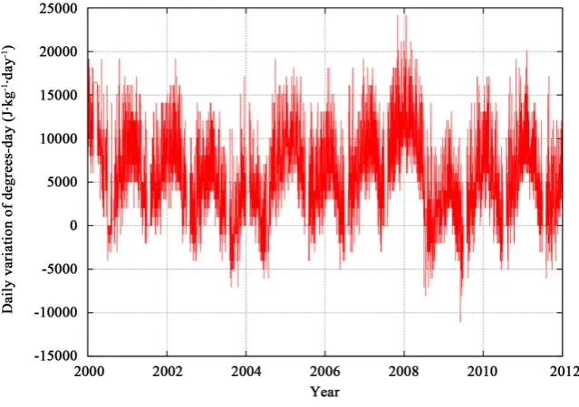
. For that we can assume a mean daily variation of air temperature in Rio de Janeiro city near to 10 (˚C⋅day−1) applied to Equation (3). The result is an estimation of the mean daily enthalpy variation, given by ∆Hdaily ≈10 10× 3(
J kg⋅ −1⋅day−1)
. The obtained valueis comparable to the average value of variation computed from observations to Rio de Janeiro city (Figure 7). This diurnal evaluation can be then multiplied by 180 days (i.e., approximately half year) in order to obtain the estimation of the inter-seasonal variation, i.e., considering the period of 6 months, started in t0.
2.2. Known Precursors of Dengue Epidemics
There are some investigations on the epidemics precursors. For instance, a comprehensible one was provided by Descloux et al. (2012) [28] which have investigated the epidemic dynamics of dengue in Noumea, that is essentially driven by the climate of previous forty years. In accord to theses authors the maximal temperature and relative humidity thresholds and their persistence were determinant in outbreak occurrences. For epidemics in Noumea, the best explicative variableswere the number of days with maximal temperature exceeding 32˚C
during Jan-Feb-Mar and the number of days with maximal relative humidity exceeding 95% during Jan. The
best predictive variables were the maximal temperature in Dec and maximal relative humidity during Oct-Nov- Dec of the previous year.
[image:5.595.87.537.597.689.2]In the present work, the enthalpy change and seasonal accumulation were used to define a predictive metabolic performance factor controlling the vector development and maturation in a tropical metropolis. Additionally, the water content into breeding sites is very important for the reproduction of vectors. The complete parametrization will be describe in the following sections, as also the model skill in explaining the Dengue outbreaks.
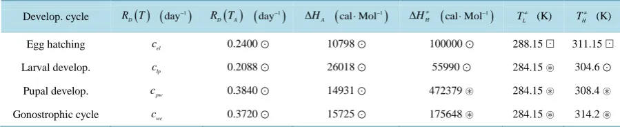
Table 1. Model parameters in function of environmental variables, associated to the enthomological enzymatic behaviour in function of air temperature. These are coefficients of the parametric performance described by the Sharpe-Schoolfield’s equation (Schoolfield et al., 1981) [51], applied to ectotherms. The coefficient values were tuned to environmental condi- tions of the Metropolitan Area of Rio de Janeiro-RJ, Brazil. The suffix A indicated the under optimum condition, TA=298.2 K
( )
.Develop. cycle RD
( )
T(
)
1
day− RD
( )
TA(
)
1
day− ∆HA
(
)
1
cal Mol⋅ − HH
≠
∆
(
1)
cal Mol⋅ − TL≠ (K) TH≠ (K)
Egg hatching cel 0.2400 10798 100000 288.15 311.15
Larval develop. clp 0.2088 26018 55990 284.15 304.6
Pupal develop. cpw 0.3840 14931 472379 284.15 308.4
Gonostrophic cycle cwe 0.3720 15725 175648 284.15 314.2
2.3. Available Data
The observational data were employed both to run and to verify the model results. First, atmospheric data observed at surface at the International Airport of Rio de Janeiro (i.e., Tom Jobin airport) are assimilated in the model, providing the necessary meteorological variables (i.e., air temperature, pressure, humidity, wind speed and direction) to the calculation of the terms of the Surface Energy Budget (SEB). Precipitation flux data (i.e., rainfall) are also obtained of local mesonet in MARJ, and assimilated by nudging, for calculations of the Surface Water Balance (SWB). A Newtonian relaxation (i.e., nudging) was used to assimilate all the atmospheric data in the model, considering a sequence of assimilation cycles of 1 hour, along all the integration time. According to Kister (1974) [29], and Haltiner and Williams (1980) [30], nudging is a dynamic method to bring the simulated variables close to the observations, without introduces shocks in the model dynamics (i.e., by filtering very short-wave along assimilation cycles). Second, Dengue fever notifications, actually available from the Brazilian public health system, were used in comparison with modelled variables.
The employed data are:
• Notification of Dengue—Used to verify the skill of hte model against observations. The data are obtained directly from the Ministério da Saúde (MS) of Brazil (SVS, 2006) [9], Secretaria de Vigilância em Saúde (SVS) and Sistema Único de Saúde (SUS, 2006) [31], and downloaded from Sistema de Informação de Agravos de Notificação (SINAN) at URL http://dtr2004.saude.gov.br/sinanweb/.
• Atmospheric data—The surface meteorological data are assimilated using cycles of 1 hour in the model. The data are obtained from a weather station installed at the International Airport of Rio de Janeiro (i.e., Tom Jobim airport). The station is maintained by the Brazilian Aeronautic Command (COMAER). The original coded data (i.e., METAR) was decode, reformatted and checked statistically (i.e., comparing each variable decoded with its mean ± 2 standard deviation threshold). Additionally, a continuous time coordinates (i.e., decimal year) was computed and added to the data. This continuous coordinates (e.g., 2015.103269290) was employed in the assimilation numerical procedure to control the flux of data in relation the internal integration time (i.e., also computed as a decimal year coordinate). The data preparation was accomplished in a Fortran-90 program created for this task. The model request some atmospheric variables which are not directly available in the observational dataset, such as the density flux of solar radiance (W⋅m−2) at surface and its components (i.e., direct, diffuse and global). To supply these variables, we have parametrized them following Flores R. et al.
(2015) [32] that optimally have fit the Iqbal solar irradiance model (IQC) (Iqbal, 1983) [21] to the observed conditions in MARJ. Indeed, some necessary thermodynamic variables (e.g., specific and relative humidity) are computed following Bolton (1980) [33].
• Hydrometeorological data-Data of precipitation sampled to each 15 minutes were also assimilated in the model. The data origin is automatic rain-gage mesoscale network (i.e., the AlertaRio system), composed by 32 weather stations dispersed on the Rio de Janeiro’s municipality area, and available from URL
http://alertario.rio.rj.gov.br/.
2.4. Dynamic Epidemic Model
Presently, there is a set of Dengue infection dynamics models for human and mosquito population as prognostic variables, or indeed stochastic models with probability of infection as the unknown, written using different levels of complexity. Below we are listing some of them:
gonotrophic cycle, in days, and the extrinsic incubation period (EIP), also in days, for the site-specific Dengue [37].
Otero et al. (2006) [23] described a dry weather model for Dengue dynamics, with temperature-dependent effects, without considering rainfall effects, directly.
Morin et al. (2010) [38] described the Dynamic Mosquito Simulation Model (DMSM), with rainfall and temperature-dependent effects, applied to a Central America tropical city.
Luz et al. (2003) [39] discussed theoretically some uncertainties to the development of Dengue models for Rio de Janeiro-RJ, Brazil, concluding that the two most important entomological parameters to be estimated in the field to compare with a numerical model of Dengue epidemics are mortality rate (of humans) and the extrinsic incubation period.
Sporleder et al. (2009) [40] proposed the Insect Life Cycle Modeling (ILCYM), a software for developing precipitation and temperature-based insect phenology models with applications for regional and global pest risk assessments and mapping, and
Lana et al. (2014) [41] with base in statistic tests with a set of prototype vector models, reccomending that future dengue models should investigate the heterogeneous levels A. aegypit of eggs through the seasons of successive years, as it may affect virus development along the years and also the occurrence of further epidemic outbreaks.
In view of the present state of development of modeling of Dengue epidemics, the following characteristics were chosen for the numerical model described in this work:
• assimilation of both variables, precipitation and air temperature, to compute the entomological parameters. In the same way, other meteorological surface variables such as the incoming solar radiation flux, the air humidity and pressure were assimilated by the Newtonian relaxation method (i.e., nudging), throughout the integration time;
• metabolic factor in function of accumulated thermodynamic variables (i.e., enthalpy, entropy, degree-day index);
• an human reinfection reservoir to implement a positive feedback in the epidemic simulation;
• four virus serotypes reservoirs and associated viremia effecting reinfection parameters and the human mortality rates due to Dengue infection; and
• free software (written in f90) and free distribution.
Consistently in the proposed model, the human mortality rate was estimated from the reinfection rate, so that this last variable can be compared with the notifications of Dengue observed. Also the metabolic factor can be activated by level of the accumulated enthalpy along the months, triggering the reproductive behaviour of the mosquitoes.
A epidemic reinfection model in function of available enthalpy
In this work a model for a infectious disease, based in a system of non-linear differential partial equations, correspondent to the temporal evolution of the dynamics of population during epidemic cycles of Dengue was implemented. The numerical implementation was done in the Fortran-90. Additionally, the assimilation of observed atmospheric data, the role of precipitation, and the effects of feedback associated with reinfections were taken in account.
The atmospheric data (air temperature, precipitation rate, specific humidity, direct and diffuse shortwave radiation flux and air pressure) were prepared and formatted as XYZ.DAT files for a 4D assimilation, imple- mented by Newtonian nudging.
The equations system was divided in three population reservoirs, which in turn were subdivided in boxes. The forecasting variables are relative fractions of the total populations, therefore the unity here represents the pandemic that has spread through the whole population and area.
Dengue virus dynamics equations
The virus population dynamics was based in the theory of exponential growing of Malthus (1798) and also in logistic growing described by Verhulst (1845) [42]. The former reference was mainly applied in population dynamics over effect of different viruses, and the later one, supposes that temporal variation of the number of infected individuals is proportional to the amount of infections, with the variation rate proportional to the fraction of non-infected population, i.e., in accord with a time scale in function of the incubation period.
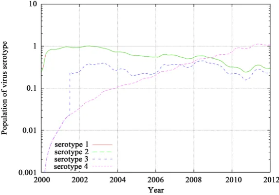
indicated by the suffix ()i in the following equation. The time of entry of each serotype also was considered in
the model, set up to MARJ, in the years 1986, 1990, 2001, and 2011, respectively. In the model, the dynamics of virus population is controlled by the following proposed equation,
(
)
4(
)
42 3
1 1
d d d d
0.01
d d d d
mut mut
i
f v i v i ji j i ij
j j
v i ir W
b v a v v v
t ν t t t = ν =ν
= − + + + + −
∑
∑
(5)where exp i v i t b τ ∆ = −
and av= −
(
1 b)
are consistency weights representing the increasing immunizationafter the time period ∆ti after the introduction of serotype ()i. τi is assumed equal to 700 days.
The first term in the r.h.s of Equation (5) represents the logistic development of the virus in the nervous system, intestine and glanders of mosquitoes, associated to the extrinsic incubation period (EIP). The second term was proposed to represent the increase of viremia associated to the infection and re-infection in the intermediate and final hosts; and, finally, the third and forth terms were introduced to represent a small effect associated with random mutation from a serotype into other.
The parameter controlling mutation from serotype j to i that is expressed by
ν
ijmut 1 107ξ
−
= × where
ξ
is a random number with uniform distribution in the range[ ]
0,1 .The air temperature was used to control the rate of incubation of the virus in the mosquitoes. In accord with the laboratory experiments of Watts et al. (1987) [43] the DENV-2 virus can be transmitted to monkeys only by
Aedes aegyptiwas retained at 30˚C or more for 25 days. Indeed, the extrinsic incubation period was 12 days for
mosquitoes at 30˚C, and was reduced to 7 days for mosquitoes incubated at 32˚C and 35˚C. Consequently, to represent the temperature-dependence of the extrinsic incubation in the present work, the parameter (νf ) was considered as a function of the incubation temperature of the mosquitoes, given by the following expression
(
)
22
35
1 1
exp
7 86400 5
C f
T
ν = − −
(6)
where TC is the environment temperature, in (˚C).
The virus quantification in laboratory involves counting the number of viruses in a specific volume of blood to determine the virus concentration. In accord with Focks and Barrera (2006) [37], studies comparing the consequences of viral titre (i.e., virus quantification) on the dynamics of endemic dengue suggest that titre, through the agency of probability of dissemination and EIP, does indeed play a role (by hypothesis).
Focks et al. (1995) [36] evaluated virus titres between 105 (i.e., a low value with partial impact on the population) and 106 (i.e., a high value with very broad impact), in relation the median infective dose (MID50%).
To update of the virus population in the numerical solution, we apply the Euler’s method in finite differences (Mesinger and Arakawa, 1976) [44], written as
( ) ( ) d ( )
d
t
t t t i
i i i
v
v v t
t
ε
+∆ =
+ ∆ (7)
where εi is the indicator function of unit that is equal to 1 if the DENV-i is present, and 0 otherwise. Mosquitoes Population Dynamics Equations
The population dynamics of mosquitoes is described from the differential equations system for the relative population dynamics of the Aedes aegypti in the aquatic and winged phases. This system allows to represent the interrelations between the different phases, in which the metamorphosis stages are related to each other throughout the different phases (i.e., the discriminant compartments of the mathematical model).
The representation in form of differential partial equations system considers different population compart- ments, that represent the successive stages of metamorphosis during the mosquito life cycle.
The equations depend on the entomological parameters, as well as environmental parameters (e.g., Yang et al., 2009 [45]). In this work, the entomological parameters were established in function of the temperature, as usual, but also in function of the estimated water availability into the breeding sites, from observed rainfall.
( )
( ) (
) ( )
( )
( ) (
) ( )
( )
( )
(
)
( )
( )
( )
( )
( )
( )
( ) ( ) (
) ( )
( )
( )
( )
1 1 2 1 2 3 2 3 d d d d d d d d d d d d e l p w ww w w
w w
E
t W t E t
t L
t E t L t
t P
t L t P t
t W
t P t i t W t
t W
t i t W t W t
t W
t W t W t
t
ψ ϕ µ
ϕ δ µ
δ σ µ
σ β µ
β γ µ
γ µ = − + = − + = − + = − + = − + = − (8) where:
(E) is the relative population of eggs, i.e., the number of eggs divided by the maximum number of eggs supported by the environmental condition.
The dynamic of the eggs population depends of the oviposition rate, ψ , which is associated with the gonostrophic cycle, fertility of female mosquitoes, and the opportune rainfall occurrences.
ϕ is the rate of eggs eclosion, from eggs to larvae The number of eggs decreases in function of a specific mortality rate, µe, in usual units of (day−1).
(L) represents the relative number of larvae, written in function of the eclosion rate
( )
ϕ ,( )
δ , a parameter controlling the pupation (i.e., the transformation of larvae into pupae), and µl, the larva mortality rate, in usual units of (day−1).(P) represents the relative population of pupae, which is function of the pupation rate
( )
δ ,σ
the rate of metamorphosis of pupa into winged mosquitoes (i.e., W1), and µp, the pupae mortality rate, in usual units of (day−1).( )
W1 represents the relative number of non-infected mosquitoes, in usual units of (day−1).
( )
W2 represents the relative number of exposed mosquitoes, of non-infectious Aedes aegypti, in usual unitsof day−1.
( )
W3 represents the relative number of winged infectious mosquitoes, after the extrinsic incubation period ofexposed wings W2 to the Dengue virus, in usual units of day−1.
( )
W is the relative number of mosquitoes Aedes aegypti, i.e., W =W1+W2+W3. Additionally, the following parameters are employed.( )
1 wi t Wβ is the rate of infection of succeptible mosquitoes by biting infectant humans, in usual units of day−1.
w
γ , the rate of transformation of W2 into W3, i.e., the inverse of the extrinsic incubation period, in usual units of day−1.
w
µ is the rate of mortality of adult mosquitoes, in usual units of day−1.
The larval behavior is controlled in Equation (8) by parameter ϕ, that depends of both the available enthalpy of the environment and of the rainfall distribution (i.e., its intensity and frequency). As proposition of this work,
ϕ is parametrized by the following
1 . b opt b H l BM H
ϕ= − ×
(9)
The first factor in the r.h.s. of Equation (9) represents the effect of the capacity of the breeding site, considered the minimum necessary volume of water to support larvae development. The variable Hb, in (m), is the height of the water into breeding site, obtained from the integration of the balance of water for the linear reservoir of surface, given the atmospheric precipitation. The scale opt
b
here proposed by the following expression
(
)
(
)
2 2 d 86400 exp d opt a a a opt a DG DG DG BMt DG t
− − = ∆ (10)
where the parameter DGaopt≈ ×3 106 was tuned out to the period of late summer in Rio de Janeiro. The first factor in r.h.s. of the BM equation is used to represent the effect of the energy of environment that is favourable to the fertility of the females of Aedes aegypti. The second effect is used to account of the oviposition of the previous year, associated with the intensity of the accumulated DG. When the oviposition was smaller in previous year, the possibility of a Dengue surge in the present year is decreased. The third factor is used to express the accumulation of energy in joules per kg and time step ∆t.
The development of the larval breeding depends on two parameters: the volume of nutrient water in the breeding and the total number of larvae present. Thus, an appropriate variable to larval development estimated rate is the concentration of larvae per unit volume of water
( )
χl in units (larvae⋅m−3), or its reciprocal, which is the specific volume of nutrient water divided by the number of larvae present, that is, the volume available to the liquid nutritional development of each larva in (m3⋅larva−1).In the Equation (9), Hb represents the height of the water accumulated in the reservoir of a typical larva breeding site, and Hopt is its optimum value, generally achieved before spill, which occurs when the rainfall
implicates t t max
b b
H +∆ ≥H . In a linear reservoir representation the ratio of water heights is equal to the ratio of
present and optimum volume of water in the breeding, i.e., b b
opt opt b b H V H V =
since Vb =Hb×Ab, with Ab is
the mean cross section area of the breeding site, constant by simplicity. The specific volumes suitable for larvae breeding can be written as
opt
opt b b
l opt
l n V
n
χ = (11)
b b
l opt
l
n V ln
χ = (12)
where nb is the total number of breeding sites in the city, and nlopt is the optimum population of larvae (integer number). The normalized difference between the larvae specific volume (χl), in (m3⋅larva−1), and this
optimum value ( opt l
χ ), i.e., χl−χlopt χlopt that can be shown to be equal the Equation (9), (dimensionless). The available water volume and feeding reservoir can constrain the larvae development. The minimal water volume for supporting the maintenance of larvae in the breeding site is approximately 7.5 10× −6
(
m3⋅larva−1)
,associated with a concentration between 46 to 60 (larvae per litre), as the optimum. The effect of the water volume in simulated breeding sites is the following: if there is too much larva (higher them 46 to 60 larva per litre), the value of ϕ becomes too small (close to zero). In this case, the larva cannot survive the competition for food and space. Thus, the interruption of the cycle of the Aedes aegypti can be emulated by the simulation. Consequently, the maximum number of larvae into a breeding has a upper limit given by the maximum volume of the reservoir.
Epidemic model on human population
The Epidemic model on human population, Equation (13), comprehends five compartments of individuals in different moments of the infection by the Dengue virus (i.e., in a similar way the exemplified models by White
et al., 2010). Here, we propose the coexistence of five classe: s t
( )
exposed population, e t( )
infected population, i t( )
infected population with transmission capacity, and r t( )
recover population. Additionally, in the present model, we have a compartment for the re-infected fraction of population, ir t( )
, generally re-infected by a different serotype.The equations are inter-related and time dependent. The progression of the infection can be controled by the following model parameters: η−1, the frequency of recuperation after a primary infection; 1
e
intrinsic incubation of the virus in the human population; and (µh), the mean rate of mortality of population for non-epidemic years. Additionally, the parameter η establishes the rate of recuperation after a re-infection by a new Dengue serotype.
The dynamic of population under dengue epidemics can be described by
(
)
(
)
(
)
d 1 d d d d d d d d d d d r s e ee h i
r
r r h r ir r
r r
i ir r
s
s i i r s
t e
s e e
t i
e i i i i
t i
k r i i i i
t r
k r i i r r
t m
i i
t
λ ω µ
λ γ µ
γ η ω µ µ
λ η ω µ µ
λ η ω µ
µ µ = − + + + + − = − − = + − − − − = − − − − = − + + − − = + (13)
The prognostic model variables for human population, in usual units of (day−1), are:
( )
s t is the relative fraction of population suceptible to a primary infection by Dengue;
( )
e t is the relative fraction of population exposed to the infection;
( )
i t is the relative fraction of population composed by infectious individuous;
( )
r
i t is the relative fraction of population reinfected by a second type serotype;
( )
r t is the relative fraction of population recuperated from Dengue infection;
( )
m t is the category of individuals that died due to Dengue fever infection.
The parameters of Equation (13), in usual units of day−1, are λ is the rate at which susceptible individuals become exposed;
e
γ is the rate at which exposed individuals become infected; η is the rate at which infected individuals become recuperated;
ω
is the susceptibility rate after infection, reinfection or recuperation;s
µ is the mortality rate of susceptible individuals,
(
µs =µh)
;e
µ is the mortality rate of exposed individuals,
(
µs =µh)
;i
µ is the mortality rate of the primarily infected individuals;
ir
µ is the mostality rate of reinfected individuous;
r
µ is the rate of mortality of recovered individuals,
(
µs =µh)
; The immunization effect after a epidemic is parametrized by4
1
1 .
ir i
i
η η ε
=
= +
∑
(14)The summation of the equations in the system (13) implies the cancellation of many opposite terms. The obtained equation can be expressed in terms of the total population (T), as follows
d d
0.
d Tr d
T
s e i i r m
t t
+ + + + + = =
(15)
This equation states the physical consistency associated to conservation of population. In the other hand, dT dt=0 is the condition of a closed population model. Since that
(
s+ + + + + =e i ir r m 1)
, the system can be closed for obtaining s as a residue.Metabolism parametrizations
natality, metamorphosis and mortality of Aedes aegypti as a function of the temperature of the breeding site. Unhappily, we cannot use directly these curves for numerical modelling purpose because they diverge from expected values under hypo and hyperthermia, i.e., outside the range of considered observations (≈8.5˚C to
≈35.0˚C). As in the MARJ, the observed maximal air temperature is frequently above 35˚C [46] [47], due to the Urban Heat Island and the anticiclonic weather condition, the practical alternative is extending the limit range of application of the curves in proper way (i.e., considering the prior technical knowledge on hypothermic and hyper- thermic inactivation effects [12]), as have been suggested by Morin (2012) [48] and Morin et al. (2013) [49].
Among others, Otero (2006) [23] has considered the metabolic rates of the mosquitoes in function of enzymatic activity, that is, depending on the poikilothermic enzymatic activity, in units of day−1, following the equation proposed by Sharpe and DeMichele (1977) [50] and Schoolfield et al. (1981) [51].
The numerical realizations considered in the present work have tested both parametrizations represented by polynomial fits [45] and Sharpe-Schoolfield’s performance equation [50] [51]. The parametrization of poikilo- thermic enzymatic activity seem more appropriate for the simulations since can be really used outside from the optimum range of temperatures, and the model approximates more of the observations.
Sharpe-Schoolfield’s equation
This subsection describes the parametrization used to represent the relative performance of ectotherms in function of the environmental temperature of breeding sites. The temperature of breeding sites is supposed to be a non-linear function of the external air temperature. The breeding sites are considered as a opened cavity to the environment, able to exchange the metabolic gases, thermal energy and water vapor by conduction and convec- tion, and acting as a reservoir for a fraction of the intercepted rainwater. The enzymatic activation/deactivation of maturation and other basal metabolisms can be associated to the relative performance of the ectotherms by equations of reaction kinetics rates (rd ), in a similar way to the proposition of Sharpe and DeMichele (1977) [50] for poikilotherm development, of Van der Have and De Jong (1977) [23] for the ectotherms in general, and also applied by Otero et al. (2006) [52] for a numerical investigation of the Aedes aegypti’s ovoposition, for a metropolis of subtropical climate.
The basal reactions kinetics rate rd298, in units of (day−1), associated with the optimum temperature
( )
298.2 K
A
T = for activation/sativation reactions, in (K). HL is the low level thermodynamic enthalpy
( 1 1
cal K⋅ − ⋅Mol− ) associated with a low temperature for half inativation of reations (TL≠); HH is the high level thermodynamic enthalpy for the high temperature for half inactivation reactions (TH≠). HA is the enthalpy level under optimum conditions (TA ~ 298.2 K).
The Sharpe-Schoolfield’s equation (Schoolfield et al., 1981) [51] can be rewritten using the formalism of a Bayesian posterior, such as the posterior distribution of the parameters (e.g., as those of kinetic reactions)
( )
(
p HT)
can be obtained by modifying the prior distribution (π
) by multiplication with the likelihood distribution of parameters (evidence). Therefore we write( )
prior:A T T
T
ρ π =
(16)
(
)
1 1likelihood: exp A A A
A H L H T
R T T
∆
= −
(17)
( ) (
( )
)
( )
posterior: p TH L H TA T p H
π
= (18)
where
( )
1(
L L) (
H H)
.p H = +p H T≠ ≠ +p H T≠ ≠ (19)
Generally, HL≠<0 and HH≠ >0. Considering the Q10 rule, i.e., for each 10˚C should the performance
increases by twice (or three times), and given the values of HA <0, TA and TL
≠, then we can
10
( )
(
)
1 ln 2 .
10
A L
L A
T T
H H
≠
≠ ≈ ∆ − −
(20)
It is common in the thermal vicinity T=TA±δT to approximate Equation (19) by p H
( )
≈1 (Salon et al., 1987) [53], specially when the linearity of Q10 rule can be supposed valid beyond the lower extreme of the range of temperatures (e.g., under reduced survivor-ship and development rates for the eggs and larval stages, peeked until favourable environmental conditions take place), or, indeed, for some asymmetrical distributions to high values, p H( )
≈ +1 p H T(
H≠ H≠)
, e.g., for pupa to wing development time (Otero et al., 2006) [23].The enthalpy HA in (J⋅mol−1) refer to the heat released or absorbed per unit of mole during a metabolic reaction, completed under thermal optimum conditions. However, the enthalpies HL≠ and HH≠ occur under less favourable conditions to the metabolic support. Therefore, the enthalpy of the enzyme kinetic reactions of the animal specimen refers to the transfer of energy that accompanying a change of state, from a reference state to a further metabolic state.
The values of enthalpy and temperatures applied here are shown inTable 1.
Bayesian statistics have been used to build robust framework for parameter estimation and uncertainty analysis in dynamical models for epidemics forecasting (Coelho et al., 2008, 2011) [54] [55]. The quality of Bayesian statistics increases with of number of samples (i.e., observations) used to defined the Likelihood, and, by product with the prior, to achieve the posterior distribution of parameters.
The Sharpe-Schoolfield’s equation [51] can be interpreted in terms of the Bayesian model statistics (i.e., as a theoretical expression of Bayes’s equation). In this case, the prior distribution can indicate the simply fact of metabolic reactions tend to increase with the temperature (e.g., as in Arrenhius’s law). The likelihood informs about the kind of distribution of the model parameters around the thermal optimum. In the Sharpe-Schoolfield’s equation, the likelihood is due to the empirical evidence, the performance have typically a Normal distribution around the optimum. The posterior distribution in function of the temperature is proportional to the product of the prior by the likelihood distribution of the parameter, resulting that Sharpe-Schoolfield’s equation follows an adjunct distribution of the exponential family, associated with a weak informative prior. Consistently, the asymmetry between the low and high temperature of a half deactivation/activation of enzyme reactions, for each site of the optimum, would result in some (positive or negative) asymmetric distribution of performance.
On the other hand, Rall et al. (2012) [56] have suggested that the temperature dependence of functional response parameters is more complex than simples Arrhenius terms, which is basically a expression of tempera- ture dependence. Thus, the biological rates depend not only on temperature, as all chemical reactions, but also on body mass. In Metabolic Theory of Ecology the Arrhenius equation is given by
(
)
(
)
0.75
0 exp I 0 0
I=I m H T−T kTT
where EI (eV) is the activation energy, k (eV∙K−1) the Boltzmann constant, T (K) is the absolute temperature,
0
T (K) sets the temperature for metabolic activation, and m is the body mass.
In the case of interaction between the dengue virus, the insect vector and human host, a minimal virus critical mass seems necessary to trigger an outbreak, since the mass of an isolated virus is extremely small in com- parison to the insect vector masses and the human host. Thus, the insertion capacity and virus proliferation in the human host will likely depend on extrinsic incubation the virus vector, which in turn, is a function of ambient temperature. This effect is implicitly considered in Equation (6).
Mortality rate for Aedes aegypti
In this work, mortality rates for different insect life stages Aedes aegypti were parameterized following the proposition Hosfall (1955), Bar-Zeev (1958) and Rueda et al. (1990). Table 2 shows the mean values of the parameters used in the model to the conditions found in the MARJ.
Open source model
The idea is that the model can receive user community contributions in a dynamic and participatory process of continuous development. Therefore, the model code is proposed as open source, available in the Internet through the Internet site of the Laboratorio de Hidrometeorologia Experimental, located in the Institute of Geosciences of the Federal University of Rio de Janeiro (IGEO-UFRJ).
Basic reproduction number
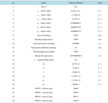
Table 2. Input constants used in the present version of the epidemic model, obtained by trial and error, considering the valid
range of values and the increase of the NSE.
cte. Name Value or reference Units
1 flag ir_ Yes -
2 cwo (mean value)
5
8.1019 10× − (s−1)
3 cw i2 (mean value) 1.1574e−8 (s
−1)
4 cw w3 2 (mean value) 5.787e−8 (s
−1)
5 µo (mean value) 0.000000012 (s
−1)
6 µl (mean value) 0.000007720 (s
−1)
7 µp (mean value) 0.000002512 (s
−1)
8 Area of breeding 0.050 (m2)
9 Breeding height (max.) 0.050 (m)
10 Leak timescale for breeding 2592000. (s)
11 Intercepted rainfall by breedings 1.0 (%)
12 Total breeding sites number 2500 -
13 Human life expectancy 2075068800.0 (s)
14 εf ageing feeding factor 2.0 -
15 βlh 4.977e−6 (s
−1)
16 η 4.24e−8 (s−1)
17 γ 9.260e−8 (s−1)
18 µi 1.1574e−14 (s
−1)
19 µir 1.1574e−12 (s
−1)
20 ωsir 1.0000e−7 (s
−1)
21 DENV-1 (arrival year) 1986.0 -
22 DENV-2 (arrival year) 1990.0 -
23 DENV-3 (arrival year) 2001.5 -
24 DENV-4 (arrival year) 2010.0 -
at the end of a extrinsic incubation period of the vector, in a large crowded conurbation (Massad et al., 2001 [58]; Luz et al., 2003 [39]).
There are some different estimations of R0 in the literature. For instance, Coelho et al.[54] have suggested the treatment of model uncertainties to obtaining a Bayesian posterior estimation of (R0), given the observa- tional evidence; Khan et al. (2014) [59] estimate for a single-strain Dengue Fever epidemics, using the model evidences (i.e., prognostic variables); and Luz et al. (2003) [39] also proposed a method to estimate R0 for Rio de Janeiro based in a Markov chain analyse and quite uninformative prior distributions.
Interestingly, Luz et al. (2003) [39] considered the risk of dengue transmission in humans proportional to density of infected vectors into the epidemic areas of lower l and high h densities. Hence, (R0) is computed starting an infectious period in the areas of low and high vector densities, called l or h. During a full incubation period, a fraction of population commutes between the two areas with daily probability δ . The expected number of secondary cases produced during the entire infectious period (R0) can be estimated by a Markov chain method as the summation on the areas of the expected daily number of secondary cases produced
(
λ λl, h)
On the other hand, considering a model of statistical correlations, Luz et al. (2003, 2008) [39] [60] have applied box-plots in comparisons of the simulated parameter performance that lead to prediction of Dengue fever epidemics outbreak (when R0>1) and disease extinction (R0≤1), for viremia in humans, mosquito mortality, and mosquito biting rate.
In the present work, we estimated R0 simply by counting the increasing number of infections in a fortnight. Breeding sites modeled by linear reservoirs
Christophers (1960) [12] characterizes the cycle of development of the Aedes aegypti mosquito, vector of the yellow fever and of the Dengue, as well as discusses qualitatively the factors of its survival, among them temperature and precipitation. These factors are classified as associated to, first, the daily cumulative develop- ment (CD), which explicitly modify the Aedes aegypti’s metamorphosis in function of the air temperature and surface precipitation, and second, the maintenance factors during the different phases of the insect life. The metamorphosis depends on the presence of water.
In particular, the oviposition and eclosion of the eggs, as well as the survival of the larva, which, after going through the pupation process achieve the stage of maturation, where the metamorphosis into pupa occurs. In all the three stages of metamorphosis mentioned above, it is known that the minimum water may be accumulated from precipitation, irrigation or accumulation for human consumption in the urban reservoirs and must be 10 (mm) or higher in height.
The Surface Energy Balance (SEB) is fundamental to the determination of the temporal evolution of atmospheric variables at surfaces (Oke, 1988) [18], particularly in cities, where urban surface topography and land cover is able to define different partitions of energy, defining different urban microclimates (e.g., as observed in down- towns with high buildings, green parks, concrete surfaces of parking, roads and even microclimates within urban dwellings). Part of net flux of energy is stored by the urban materials and buildings, providing a 24 hours cycle of hysteresis between temperature and the net flux of radiation (Ferreira et al., 2013) [61].
According to Piovezan (2009) [62], the predominant breeding sites for the development of the aquatic phase of the mosquito are presented in three types: dishes and pots for plants, cans, pots and flasks, and other types of removable receptacles. Additionally, it is interesting to include in this list: open water tanks, abandoned pools, big cans, flower pots in cemeteries [23], refuse dumps etc.
Hypothetically, places considered prone to mosquito aquatic phase development are those subject to recept a partial flux of incoming water during precipitation vents (i.e., a smoothed flux), with thermal conditions around to the most favourable thermal conditions (i.e., close to the optimum), obtained with the Mosquito’s oviposition preference by partially shadowed sites. With that in mind, the breeding sites in the MARJ most propitious to the development of the aquatic phase of Aedes aegypti are those under partial shadowing and with only partial interception of rainfall.
Once the reservoirs of water of the urban breeding sites are essentials to the aquatic phase of the mosquito behavior, the data analysis of precipitation and relative humidity were accomplished in detail. The goal was quantifying the model sensibility in relation to these variables. As result, we observed that a large number of weak to moderate rainfall events, alternated with hot sunny periods, can be most favourable to aquatic develop- ment of larvae than the occurrence of some few strong rainfall events of equivalent height of water. By hypothesis, with rain interspersed with periods of sun the breeding sites can lose water due to evaporation, but not in the potential rate due to the partial shadowing conditions inside them.
A Linear Reservoir Model (LRM) was used to represent the average dynamics of breeding sites. To supply the water for breeding reservoirs the atmospheric precipitation was assimilated by nudging. The lost of water due to evapotranspiration and leaks was also represented in the modelled breeding sites. The loss is parametrized by the sum of the estimated Potential Evapotranspiration (PET) plus a smaller amount reservoir leaking, in the form of a simplified Surface Water Balance (SWB) (Grimmond et al., 2002 [63]; Karam et al., 2010 [47]).
The Potential Evapotranspiration (PET) was obtained with the known Penman’s Combination Method (Penman, 1948 [64]; Thom e Oliver, 1977 [65], and Monteith and Unsworth, 2007 [66]). The calculation of the PET depends on the data assimilation of the net irradiance flux (Rn).
In this work, for representing the urban breeding sites we use the LRM and the PET, provided modelled data of the net irradiance flux (Flores Rojas et al., 2015) [32]. In a way similar to doing in simulations of WSB to natural surfaces, for the urban breeding sites the variation of the water volume along the time was given in function of the observed influx and lose of water. The modelled recharge occurs during atmospheric precipi- tation events due to the interception, modelled by a small fraction of the total rainfall, estimated near to 1% for Rio de Janeiro metropolis. Due to the shadowing condition of the breeding sites, it is also considered a fraction of the PET calculated (i.e., equal to 60%) to simulate the evaporative conditions found in the breeding sites.
The idea of using linear reservoirs to simulate the breeding site is well known in the literature. For instance, a application of SWB and SEB for modelling breeding sites for larvae and pupae development, in function of the observed temperature and precipitation, was comprehensively described by Sporleder et al. (2009) [40]. In this case, the researchers obtained the spatial and temporal distributions of the vector population on Australia territory, in a GIS platform. Differently, no rainfall was considered in Otero’s temperature-dependent model for model the summer surges of Dengue fever, for Buenos Aires city, in Argentina, where the climate is subtropical, with cold and rainy weather in winters (Otero et al., 2006) [23]. In the Otero’s model, the oviposition presents hysteresis behaviour to the seasonal variation of the air temperature. That is not the expected case of a tropical city as the Rio de Janeiro’s metropolis, where the diurnal variation of temperature is commonly larger than the seasonal variation (i.e., as typical of a tropical climate city).
Goodness-to-fit statistics
Lana et al. (2014) [41] have applied several goodness-to-fit statistics to verify their model performance, e.g., statistics based on the log-likelihood functions for transition probabilities of fitted Markov chains, e.g., as the
Akaike Information Criterion (AIC).
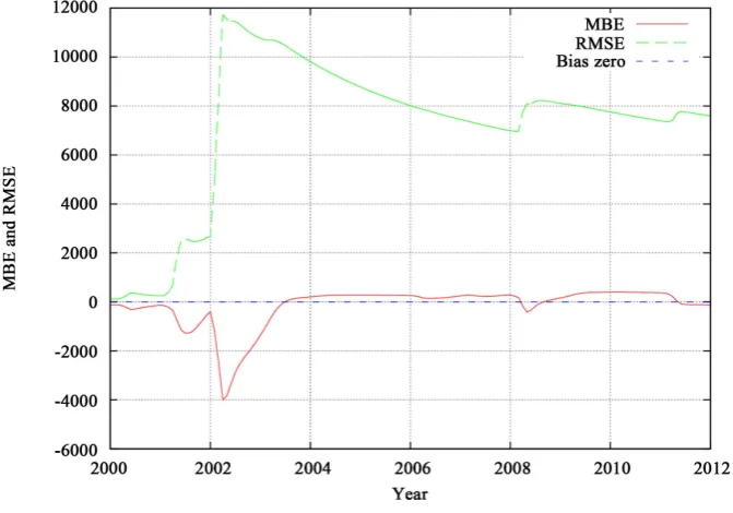
In this work, a set of statistical estimators were applied to verify the model performance and tuning the model parameters. These scalar accuracy measures are the Mean Absolute Error (MAE), the Mean Squared Error
(MSE), the Root Mean Squared Error (RMSE), the Coefficient of DeterminationR2, and the Nash-Sutcliffe Efficiency (NSE), as recommended by Nash and Sutcliffe (1970) [72], Singh et al., (2005) [73], Moriasi et al. (2000) [74], and Wilks (2006) [75].
3. Results
The analysis of atmospheric observations and Dengue fever notifications were performed, as well as, simula- tions and parameter tuning.
First, a simple statistical analysis was accomplished on dengue notification data from SUS.
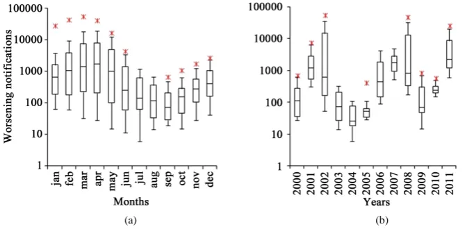
The major epidemic events in the analysis period are shown inFigure 1 andFigure 2. Box plots permit to examine the distribution of quantiles associated with the epidemics (Figure 3).
The threshold number for establishing the beginning of epidemics seems to be very small. The variability of notifications (Figure 1) becomes very evident by the use of a logarithmic scale (Figure 2). Therefore, what can be observed is the environmental conditioning, defining not only the surge itself, but also its severity, as can be evidenced by the wide distribution of the number of reports of worsening by dengue fever in the dataset.
The three bigger epidemics of Dengue in the period 2000-2011, occurred in the years of 2002, 2008 and 2011 (Figure 1andFigure 2).
Based in absolute values of number of Dengue notifications, the month of March is the month with biggest number of cases, followed by February, April and January. Although the month of March presents a larger absolute value in the notified Dengue cases, the month of April shows a larger epidemic volume, occurring a decline in the number of cases from April on.
Dengue shows a seasonal aspect, with a cyclic tendency of the epidemic varying from August to April, suggesting that the monthly distribution of the cases varies in function of the seasons of the year, with a probable chronological delay addressed to the period comprehended between the mosquito life cycle and the appearance of clinical characteristics in human organisms, this delay lasts an average of 40 to 45 days.
The shape of the envelope shown inFigure 1 seems to suggest a nearly periodic cycle of 4 to 6 years.
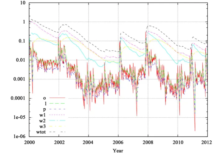
Figure 1. Time evolution of Dengue epidemics in the MARJ between Jan/2000 and Dec/2011.
[image:17.595.154.477.303.481.2]Data source: SUS-Brazil.
Figure 2.Time evolution of Dengue epidemics in the MARJ between Jan/2000 and Dec/2011, plotted with the same data used in Figure 1, but using logarithmic scale for number of occurren-
ces. Source of raw data: SINAN-net/SUS.
(a) (b)
Figure 3. Box plots of notified cases of Dengue fever reported for the Rio de Janeiro city durante
[image:17.595.147.482.530.695.2]