Munich Personal RePEc Archive
Evaluating the Precision of Estimators of
Quantile-Based Risk Measures
Cotter, John and Dowd, Kevin
2007
Online at
https://mpra.ub.uni-muenchen.de/3504/
Evaluating the Precision of Estimators of Quantile-Based Risk Measures
By
Kevin Dowd and John Cotter∗
Abstract
This paper examines the precision of estimators of Quantile-Based Risk Measures
(Value at Risk, Expected Shortfall, Spectral Risk Measures). It first addresses the
question of how to estimate the precision of these estimators, and proposes a Monte
Carlo method that is free of some of the limitations of existing approaches. It then
investigates the distribution of risk estimators, and presents simulation results
suggesting that the common practice of relying on asymptotic normality results might
be unreliable with the sample sizes commonly available to them. Finally, it
investigates the relationship between the precision of different risk estimators and the
distribution of underlying losses (or returns), and yields a number of useful
conclusions.
Keywords: Value at Risk, Expected Shortfall, Spectral Risk Measures, Moments,
Precision.
JEL Classification: G15
May, 2007
∗
1. INTRODUCTION
Since they arose in the early 1990s, risk managers have come to rely heavily on
models that forecast the risks associated with financial portfolios. Often known as
Value-at-Risk (VaR) models, these models in fact can and sometimes do forecast the
complete density functions of prospective financial losses (or, equivalently, financial
returns). The outputs of these models can then be used to forecast a variety of
different measures of financial risk: these include measures such as the VaR and the
Expected Shortfall (ES), but also families of risk measures such as coherent, spectral
and distortion risk measures.1 However, these risk forecasts are inevitably open to
error – the density functions might be misspecified (giving rise to model risk), and
model parameters are unknown, which forces risk managers to rely on estimated
parameters and exposes them to parameter risk – and it is therefore important that risk
managers have some idea of the precision or accuracy of the forecasts on which they
are relying.
This paper investigates this issue, and addresses three particular questions
related to the precision of risk forecasts:
• How can we estimate the precision of different risk forecasts? This is not a new
question, and there is considerable literature on it (see section 3 below).
However, as we shall see, existing approaches are limited in a number of ways,
and the present paper proposes a more flexible Monte-Carlo approach that is
free of many of the limitations of the approaches proposed so far.
• What do we know of the distributions of estimators of financial risk measures?
In fact, we know from existing statistical theory that these distributions are
asymptotically normal, and practitioners often rely on such asymptotic results as
practical short-cuts. Unfortunately, we do not know how large the sample sizes
must be for asymptotic results to be taken seriously. Thus, investigating the
finite sample properties of these estimators is of considerable practical
importance.
• What can we say about the relationship between the precision of risk forecasts
and the underlying loss (or return) density function? So, for example, can we say
1
anything about how estimates of precision might be affected by factors such as
skewness or tail heaviness in the underlying loss distribution? This is a very
difficult question to answer in a general way, but we suggest a procedure that
provides some useful insights into these issues and into related questions such as
the relative precision of estimators of different financial risk measures.
This paper is organized as follows. Section 2 discusses the risk measures to be
considered: the VaR, the Expected Shortfall, and the Spectral Risk Measures
(SRMs).2 Section 3 discusses the existing literature on the precision of estimators of
financial risk measures, and section 4 discusses alternative estimators of precision.
Section 5 sets out our methodology for evaluating the precision of our risk-measure
estimators, and section 6 looks into the difficult issue of the relationship between the
precision of these estimators and the underlying loss (or return) distribution. Section 7
concludes.
2. ALTERNATIVE RISK MEASURES
Suppose our underlying random variable is the realised daily loss (which is positive
for an actual loss, and negative for a profit) on a portfolio. If the confidence level is
α
, our first risk measure is the VaR at this confidence level, i.e.:α α q
VaR = (1)
where qα is the
α
-quantile of the loss distribution. The VaR is the most widely usedfinancial risk measure, but has been heavily criticized in recent years for some of its
properties (e.g., its lack of subadditivity; see, e.g., Artzner et al., 1999). Note,
therefore, that the VaR is defined in terms of a conditioning parameter, the confidence
level, the value of which usually needs to be specified – more or less arbitrarily – by
the user.
Our second risk measure is the ES, which can be defined as the average of the
worst 1−α of losses. In the case of a continuous loss distribution, the ES is given by:
2
− = 1 1 1 α α
α q dp
ES p (2)
The ES gives equal weight to each of the worst 1−α of losses and no weight to any other observations. The ES is superior to the VaR in a number of respects (e.g., it is
subadditive and coherent). However, the ES is specified in terms of the same
conditioning parameter as the VaR and, as with the VaR, there is often little to tell us
what value this parameter should take.
Our third measure is a Spectral Risk Measure (SRM). Following Acerbi
(2002), consider a risk measure Mφ defined by:
=
1
0
) (p dp q
Mφ pφ (3)
where φ(p) is a weighting function defined over p, the cumulative probabilities in the
range between 0 and 1. Borrowing from Acerbi (2004, proposition 3.4), the risk
measure Mφ is coherent if and only if φ(p) satisfies the following properties:
• Positivity: φ(p)≥0, i.e., weights are always non-negative.
• Normalisation: =
1
0
1 ) (p dp
φ , i.e., weights sum to one.
• Increasingness: φ′(p)≥0, i.e., higher losses have weights that are higher than
or equal to those of smaller losses.3
We now need to specify a suitable weighting function φ(p), and a good
choice is the following exponential function:
k p k e ke p − − − − = 1 ) ( ) 1 (
φ (4)
3
where the coefficient k is the user’s degree of absolute risk aversion. The function
) (p
φ can also be interpreted as the user’s risk-aversion function. The user’s risk
aversion means that higher losses attract higher weights than small losses, and the
more risk-averse the user, the more rapidly the weights will rise. The risk measure
itself then can then be obtained by substituting (4) into (3), viz.:
− − − − − − = − = 1 0 1 0 ) 1 ( 1
1 e e q dp
ke dp q e ke
M k kp p
k
p k p k
φ (5)
Thus, an SRM has the attractive property that it takes account of the user’s risk
aversion. Furthermore, an SRM based on an exponential risk-aversion function is
predicated on a single conditioning factor, the user’s degree of absolute risk aversion.
And, unlike the earlier conditioning parameter, the value of this parameter is unique
(i.e., because it is determined by the user’s risk-aversion).
3. EXISTING LITERATURE ON THE PRECISION OF RISK ESTIMATORS
Naturally, we never actually know the values of our risk measures in practice, because
the parameters of the loss distribution will be unknown. (This is true even in the
favourable unlikely case where the form of the distribution itself is known, but we
will ignore this issue here.) We must therefore work with estimates of these
parameters, and this means that we must deal with estimators of our risk measures.
(We will henceforth call these “risk estimators” for short, to avoid the correct but
ungainly term “risk-measure estimators”.) This then raises a key question: how can
we evaluate the precision – or more loosely, the accuracy – of risk estimators?
Before we begin to answer this question ourselves, we should first consider
the answers provided in established literature, and the principal findings of 22 studies
in this literature are summarised in Table 1.4 This shows that existing studies differ
enormously in how they have addressed the precision issue. It also shows that many
of these studies are limited in one way or another:
• The majority of them only apply to one risk measure, and typically the VaR.
4
• Some approaches are limited to a single distribution (e.g., Jorion (1996) and
Chappell and Dowd (1999) require that losses be normal).
• A number of approaches only give estimates of standard errors (i.e., and do not
give confidence intervals). However, as discussed in the next section, standard
errors can give misleading impressions of the precision of risk estimators.
• A considerable number of approaches are based on asymptotic theory, and
asymptotic results might not be appropriate with the sample sizes that
practitioners often have to work with.5
Insert Table 1 here
Some studies also report results on the relative precision of different risk estimators.
For example, several studies find that VaR and ES estimators have comparable
precision when loss distributions are normal or close to normal, but ES estimators
decline in precision relative to VaR estimators as tails become heavier (e.g., Yamai
and Yoshiba (2002), Acerbi (2004)). However, such findings are essentially
illustrative and one of the purposes of the present study is to shed more light on these
and related issues.
4. PRECISION ESTIMATORS AND THE DISTRIBUTION OF RISK
ESTIMATORS
We also we need to consider how to estimate precision itself. One obvious way to do
so is to estimate the standard error (SE) of a risk estimator. The SE is helpful in its
own right as a (rough and ready) estimate of precision, and can also be used to
construct confidence intervals using textbook formulas. However, as Yamai and
Yoshiba (2002) note, comparisons of the SEs across a set of different risk measures
are complicated by the fact that the different risk measures considered typically have
different values. For example, the SE for risk measure A might be larger than the SE
for risk measure B, so in such circumstances it does always make sense to say that
5
risk measure A is estimated less precisely than risk measure B? The answer is
obviously ‘no’: the first risk measure might have a much bigger value than the
second, and its SE might be only marginally bigger than that of the second risk
measure. In this case, the ‘absolute’ SE for A would be larger than that of B, but in
relative terms – that is, relative to the value of the risk measure itself – A is estimated
more precisely than B. We should therefore estimate precision taking account of the
estimated value of the risk measure, and can do so by working with a ‘standardized’
SE rather than an ‘absolute’ SE, i.e., we work with the SE divided by a point estimate
of the relevant risk measure.6
A second precision estimator is a confidence interval. A confidence interval is
often more helpful than an SE because it can give a more ‘complete’ picture of
precision: it can take more account of the distribution of risk estimators and so allow
for factors such as asymmetries, heavy-tails, etc., that can cause the SE to give a
‘misleading’ impression of precision. However, as with SEs, comparison of ‘raw’
confidence intervals can be problematic when the risk measures themselves have
different values, so we work here with confidence intervals in standardized form, i.e.,
with ‘raw’ confidence intervals divided by point estimates of risk measures.
It is also useful to examine the related issue of the distribution of the risk
estimators themselves. In fact, it is well-known in the statistical literature that linear
combinations of order statistics are asymptotically normally distributed (see, e.g.,
Stiegler (1974), Mason (1981)), and this result implies that estimators of all three of
our risk measures should be asymptotically normal. However, knowing that the
distribution of risk estimators approaches normality in the limit as our sample size
gets large does not tell us whether it is safe to assume that they are normally
distributed for any given (finite) sample size: we don’t know how quickly the
estimators converge to normality as the sample size increases. Hence, if we are
thinking of using asymptotic results, it is prudent to check if the distribution of risk
estimators is ‘close enough’ to normality to allow those results to apply.
Such information is also important in determining the usefulness of several
alternative precision estimators:
6
• The SE as a precision indicator implicitly presupposes that the distribution is
symmetric, and where distributions are asymmetric, we really need an
alternative indicator that allows for this asymmetry.
• The SE is often used as an input to textbook formulas for confidence intervals,
but this practice is only defensible if the underlying risk estimators are suitably
‘well-behaved (e.g., symmetric, and normally or t distributed), and this
‘well-behavedness’ condition might not hold empirically. Where such assumptions do
not hold, we should use properly constructed confidence intervals (e.g., Monte
Carlo-based intervals) instead.
5. METHODOLOGY
We wish now to get some sense of how the precision of risk estimators varies across
the different types of risk measure. However, this task is complicated by: (a) the
variety of precision estimators available; (b) the possibility that results will depend on
sample size and/or the conditioning parameter; and (c) the likelihood that results will
depend on the underlying loss distribution (e.g., results might depend on the skewness
or kurtosis of this distribution). Handling (a) and (b) is relatively straightforward, but
dealing with (c) is more difficult because we cannot search over every plausible loss
distribution. We therefore need a meaningful way to restrict our search, whilst also
attempting to draw out conclusions of (hopefully) more general validity.
We also need some way of organising the search. One reasonable approach is
based on the principle that we start from a simple benchmark distribution and get
some sense of the precision of the different risk estimators in this benchmark case. A
simple and well-understood (and therefore natural) benchmark is a standard normal
distribution. We then need some way of generalising from this benchmark case to see
how generalisation might affect our results. We would suggest thinking of
generalisation in terms of the successive relaxation of the moment restrictions implied
by our chosen benchmark (i.e., that the mean should be 0, the variance should be 1,
the skewness should be 0 and the kurtosis should be 3). We initially generalise by
relaxing the first and second moment (i.e., mean and variance) restrictions, and so
move from a standard normal to an unrestricted normal. After this, we generalise
kurtosis) restrictions. Naturally, we recognise that there are different ways of relaxing
these moment restrictions, and there is no uniquely ‘best’ way to do: all we can do
here is suggest a plausible procedure and then regard any conclusions we draw from
this analysis as tentative hypotheses that would be subject to confirmation (or
rejection) by later studies.
The precise approach is as follows. We first select a range of sample sizes, and
in this paper we choose n equal to 250, 500, 1000 and 2000. These values correspond
to sample sizes of 1, 2, 4 and 8 trading years at 250 trading days to a year: this is a
good range, because risk practitioners would not usually work with sample sizes that
are less than 1 trading year or more than 8 trading years. In fact, many practitioners
would work with sample sizes of 250 or 500, so it is the shorter end of the sample
range that we should mainly be interested in. We then select some illustrative
parameter values for our risk measures (i.e., we choose values for the confidence level
for our VaR and ES risk measures, and values for the coefficient of absolute risk
aversion in the case of our SRM). We chose fairly standard confidence-level values of
90%, 95% and 99%, and we chose a fairly wide range of ARA values equal to 5, 25
and 100. Having made these calibrations, we then implement the following
three-stage procedure.
•Stage One: We select a standard normal benchmark and assume that losses are
standard normal. We then estimate the precision of our different risk estimators
using our two different precision estimators across the range of selected sample
sizes, and thence evaluate how the precision of our risk estimators in the standard
normal case changes as we alter the way that precision is measured and as we vary
the sample size.
•Stage Two: We then consider how our results might change in the face of changes
in the mean µ and standard deviation σ of portfolio losses. More specifically,
we compare the cases of (µ=5,σ =1) and (µ =0,σ =5) against our standard
normal benchmark (µ =0,σ =1). The former gives an example of a non-standard
mean, and the latter an example of a non-standard variance. Given that the normal
is ‘well-behaved’ and well understood, these two alternative cases should suffice
to give a fairly complete picture of the sensitivities of results to changes in µ and
•Stage Three: Given that the normal restricts the skewness and kurtosis to 0 and 3
respectively, we now select two convenient cases involving skewness and excess
kurtosis. More particularly, the impact of skewness is examined by selecting a
two-part normal (2PN) distribution, where the latter is calibrated to produce a
skewness of about 0.492.7 Comparing this 2PN against the standard normal gives
us a comparison between a distribution that has no skew and one that has a fairly
pronounced skew, and this range of skewnesses encompasses those commonly
observed in financial returns. The impact of excess kurtosis is captured by a
zero-mean, unit-standard deviation t distribution with 5 degrees of freedom.8 This
distribution has a kurtosis of 9, which is higher than the kurtoses usually reported
for financial returns. Thus our comparison of the t and the standard normal implies
that we are comparing a range of kurtoses from 3 to 9, and this range includes the
kurtoses usually found for financial returns.
All calculations were carried out using parametric Monte Carlo simulation
with 10000 simulation trials in each case: we run 10000 trials under the specified loss
distribution, and estimate the various risk measures from the ‘sample’ order statistics
generated in each trial;9 we then estimate the (standardised) SE and (standardised)
confidence interval from the 10000 sets of ‘sample’ risk estimates obtained in this
way.
7
The 2PN can be represented in various ways, but the particular distribution chosen here is the (µ,σ1,σ2) representation of the 2PN with µ=0, σ1=1.3 and σ2 =0.65. These parameter values ensure that our 2PN has zero mean, unit variance, a skewness of about 0.492 and a ‘small’ (and hopefully negligible) excess kurtosis (equal to 0.148). For more on this distribution, see John (1982).
8
This distribution has a pdf equal to (v−2)/v times the pdf of a Student-t with v degrees of freedom (taken in our calibrations to be 5). This distribution has zero mean, unit variance, zero skew, and (provided v>4, which is necessary for the kurtosis to exist) a kurtosis equal to 3(v−2)/(v−4). For more on the Student-t, see Evans et alia (2000, p.180).
9
To be more precise: if we want the quantile or VaR at the, say, 90% confidence level, and we have 1000 loss observations in our simulated sample, we follow the usual practice and take this quantile/VaR estimate to be the 101st highest loss observation; and we then take the ES estimate as the average of the 100 highest loss observations. More generally, for a confidence level α and sample size
6. RESULTS
Stage One: Standard Normal Losses
We begin by examining the distributions and precision measures of our risk
estimators under standard normality.
VaR results
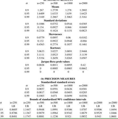
The results reported in Table 2 suggest that the standard normal VaR estimators have
the following properties:
• Their means rise with α and are invariant to n, as expected.
• Their standard errors rise with α and fall with n, as expected.
• Their skewnesses tend to be positive, rise with α, fall with n, and go to zero as
n gets large.
• Their kurtoses tend to exceed the normal kurtosis (i.e., 3), rise with α, fall with
n, and approach 3 as n gets large.
• Their Jarque-Bera (JB) test results are not supportive of normality, except where
α is low and n high.
• The precision results indicate no clear pattern as α rises (which is perhaps a little surprising given that we might have expected that precision would
consistently fall with the high values of α that we are considering), but they do indicate that precision rises with n (which is what we would expect).
Insert Table 2 here
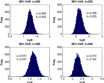
The third, fourth and fifth findings suggest that VaR estimators tend to
normality as n gets large, but they also approach normality more slowly as α gets larger. This impression is confirmed by Figure 1, which shows histograms for the
90% and 99% VaRs for sample sizes of 250 and 500. This Figure indicates that the
99% VaR estimators are notably non-normal, especially for the smaller sample size:
they also indicate that the convergence of 99% VaR estimators to normality is slow.
This suggests that, with the sample sizes often available, practitioners would be
distributed, i.e., in particular, they should be wary of using results based on
asymptotic normality theory.
Insert Figure 1 here
This conclusion also has two other useful corrolaries. (1) If the distribution of
VaR estimators is not symmetric, then practitioners should not use the SE as a
precision measure. (2) If the distribution of VaR estimators is not normal, then
practitioners should be careful about estimating VaR confidence intervals by inserting
estimates of SEs into textbook formulas for confidence intervals, because those
formulas might not apply.
ES results
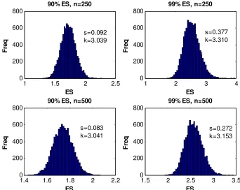
The ES results reported in Table 3 and illustrated in Figure 2 are similar to the VaR
ones in most ways (e.g. they generally exhibit a positive skewness, have comparable
precision, etc.) and the only other noteworthy features are the following:
• The skewness, kurtosis and JB results usually suggest that ES estimators are a
little ‘closer to normal’ than the earlier VaR estimators.
• The precision measures are now ‘well-behaved’ in the sense that they indicate
that precision falls with α as well as rises with n. Taken together, these first two bullet points suggest that ES estimators are a little ‘better behaved’ than VaR
estimators.
• Most importantly, in this standard normal case, the precision of ES estimators is
of much the same order of magnitude as that of VaR estimators.
Insert Table 3 here
Insert Figure 2 here
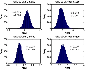
SRM results
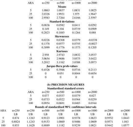
The corresponding results for the SRM risk measure are shown in Table 4 and
illustrated in Figure 3. These suggest that the ARA coefficient plays much the same
estimators of all three risk measures have similar precision. These results also
suggest that SRM estimators tend to be a little bit closer to normal than the ES
estimators, and are certainly closer to normal than the VaR estimators.
Insert Table 4 here
Insert Figure 3 here
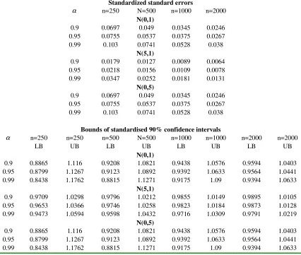
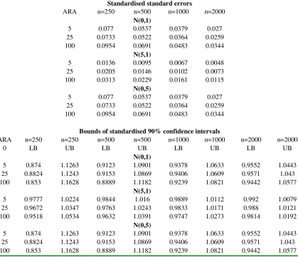
Stage Two: Non-Standard Normal Losses (Impact of Mean and Variance)
Having established results for the benchmark case where losses are standard normal,
we now investigate how results might change as we allow for changes in the mean
and standard deviation. To do so, we compare results based on three hypothetical sets
of parameter values: µ =0 and σ =1 (our benchmark case); µ=5 and σ =1; and
0 =
µ and σ =5. A comparison of the first and second cases allows us to investigate
the impact of a change in µ; and a comparison of the first and third cases allows us to
investigate the impact of a change in σ .
Our results are clear. For all risk measures, changes in the mean and/or
standard deviation have no impact on the higher moments of the distribution of risk
estimators (and therefore have no impact on the skewness, kurtosis and JB test
results). Furthermore, changes in the mean and standard deviation have the impacts
we might expect on a priori grounds. More specifically, we get the following results,
given in Table 5 to 7:
An increase in µ:
• impacts the means of the risk estimators pari passu (in the cases of VaR and ES)
or close to pari passu (in the case of the SRMs);
• has a ‘small’ negative impact on the standard error, which declines as n gets
larger; and
• has a ‘moderate’ widening impact on the confidence intervals, and this impact
declines as n gets larger.
• leads to major increases in the means of the risk estimators, and these increases
are of broadly the same order of magnitude across the different risk measures
and are greater for higher α; and
• leads to the same precision estimates as in the standard normal case. Thus
precision estimators are ‘well behaved’ and are of broadly the same magnitude
across the risk measures.
Drawing these findings together, perhaps the most significant conclusion is
that for normally distributed losses, estimates of precision are of much the same order
of magnitude across the different types of risk estimator.10
Insert Table 5 here
Insert Table 6 here
Insert Table 7 here
Stage Three: Non-Normal Losses (Impact of Skewness and Kurtosis)
Impact of skewness
The skewness results are presented in Tables 8. These are presented as the relevant
2PN estimate divided by the corresponding standard normal estimate. This format
makes it easy to see the impact that skewness makes. These results paint a very clear
picture, i.e., introducing skewness:
• has a notably positive impact on the standard errors;
• has a negligible effect on the width of the confidence intervals;
and these results hold for all risk estimators.
Insert Table 8 here
Impact of kurtosis
Tables 9 give the corresponding kurtosis results, in this case expressed as the ratio of
the precision estimates generated under our specified t distribution divided by the
10
corresponding estimators generated under the standard normal. The main highlights
are:
• Risk estimators under the t-distribution are always less precise than their
counterparts under standard normality, and this suggests that excess kurtosis
makes risk estimators less precise.
• Increasing the conditioning parameter (i.e., depending on the risk measure, the
confidence level or the degree of risk aversion) makes risk estimators under
the heavy-tailed distribution less precise, relative to their counterparts under
standard normality.
• By and large, the ratios are somewhat higher for the ES and SRM estimators.
This suggests that tail heaviness has a greater (though not much greater)
deleterious effect on the precision of ES and SRM estimators than on the
precision of VaR estimators.
Insert Table 9 here
7. CONCLUSIONS
This paper addresses three main issues. The first is the question, how can we estimate
the precision of different risk estimates? Various methods have been suggested in the
existing literature, but many existing methods are subject to significant limitations:
they apply to one risk measure only (typically the VaR), or are limited to specific
distributions (e.g., the normal distribution), or only give estimates of standard errors
(i.e., and don’t give estimates of confidence intervals), or rely on asymptotic theory
(which may not be appropriate empirically). We suggest an approach based on Monte
Carlo simulation that is free of the above limitations.11
The second issue addressed is the distribution of risk estimators. We know
from existing statistical theory that the distribution of risk estimators is asymptotically
normal. However, this theory does not tell us how quickly estimators converge to
11
normality, and the results presented here indicate that this convergence is sufficiently
slow that practitioners working with 1-day forecast horizons will often not have
samples long enough for them to invoke asymptotic normality. Thus, for most
practical purposes we cannot rely on risk estimators to be normally distributedwith
the sample sizes often available. 12
The final issue addressed is the question of how the precision of risk
estimators might be affected by the underlying loss distribution. This is a very
difficult question to answer in a general way, but we suggest a procedure that
highlights the moments of the loss distribution: we start with a standard normal which
restricts what each of the first four moments should be; we then relax each of these
moment restrictions in turn and see what effect the relaxation has on our precision
estimates. This procedure generates some insightful results, including the following:
• When the loss distribution is normal, estimators of all three risk measures have
similar precision.
• The impact of skewness on precision depends on how we measure precision:
introducing skewness has a noticeable positive impact on (standardized)
standard errors, but no notable impact on (correctly estimated standardized)
confidence intervals.
• Introducing excess kurtosis into the loss distribution has the effect of making all
risk estimators less precise than they were, and it reduces the precision of ES
and SRM estimators somewhat more than it reduces the precision of VaR
estimators.
Of course, we recognise that these results were obtained for specified distributions,
and it is possible that a different set of distributions might lead to somewhat different
conclusions. We therefore offer these conclusions as tentative hypotheses – albeit
plausible hypotheses – that other researchers might wish to investigate further.
12
REFERENCES
Acerbi, C., 2002, Spectral measures of risk: a coherent representation of subjective
risk aversion, Journal of Banking and Finance, 26, 1505-1518.
Acerbi, C., 2004, Coherent representations of subjective risk-aversion, Pp. 147-207 in
G. Szegö (Ed,) Risk Measures for the 21st Century, (Wiley: New York).
Artzner, P., F. Delbaen, J.-M. Eber, and D. Heath, 1999, Coherent measures of risk,
Mathematical Finance, 9, 203-228.
Butler, J. S., and B. Schachter, 1998, Estimating Value at Risk with a precision
measure by combining kernel estimation with historical simulation, Review of
Derivatives Research, 1, 371-390.
Chappell, D., and K. Dowd, 1999, Confidence intervals for VaR, Financial
Engineering News, March 1999, pp. 1-2.
Chen, S. X., 2005, Nonparametric estimation of expected shortfall, mimeo, Iowa State
University.
Chen, S. X., and C. Y. Tang, 2005, Nonparametric inference of value at risk for
dependent financial returns, Journal of Financial Econometrics, 3, 227-255.
Cotter, J., and K. Dowd, 2006, Extreme quantile-based risk measures: an application
to futures clearinghouse margin requirements, Journal of Banking and
Finance, Forthcoming.
Dowd, K., 2000, Assessing VaR accuracy, Derivatives Quarterly, 6 (3), 61-63.
Dowd, K., 2001, Estimating VaR with order statistics, Journal of Derivatives, 8,
23-30.
Dowd, K., 2005, Measuring Market Risk, 2nd edition. (Wiley: Chichester and New
York)
Evans, M., N. Hastings, and B. Peacock, 2000, Statistical Distributions, 3rd edition.
(Wiley: Chichester and New York)
Frey, R. and A. J. McNeil, 2002, VaR and expected shortfall in portfolios of
dependent credit risks: conceptual and practical insights, Journal of Banking and
Finance, 26, 1317-1334.
Giannopoulos, K., and R. Tunaru, 2004, Coherent risk measures under filtered
historical simulation, Journal of Banking and Finance, 29, 979-996.
Gourieroux, C., and W. Liu, 2006, Sensitivity analysis of distortion risk measures,
Gouriéroux, C., Scaillet, O. and J. P. Laurent, 2000, Sensitivity analysis of values at
risk, Journal of Empirical Finance, 7, 225-245.
Inui, K., and M. Kijima, 2004, On the significance of expected shortfall as a coherent
risk measure, Journal of Banking and Finance, 29, 853-864.
John, S., 1982, The three-parameter two-piece normal family of distributions and its
fitting, Communications in Statistics – Theory and Methods, 11, 879-885.
Jorion, P., 1996, Risk2: Measuring the risk in value at risk, Financial Analysts Journal
52, November/December, 47-56.
Kendall, M., and A. Stuart, 1972, The Advanced Theory of Statistics, Vol. 1:
Distribution Theory, 4th edition. (Charles Griffin and Co. Ltd: London)
Manistre, B. J., and G. H. Hancock, 2005, Variance of the CTE estimator, North
American Actuarial Journal, 9, 129-156.
Mason, D. M., 1981, Asymptotic normality of linear combinations of order statistics
with a smooth score function, Annals of Statistics, 9, 899-908.
Mausser, H., 2001, Calculating Quantile-based Risk Analytics with L-estimators,
Algo Research Quarterly, 4, 33-47.
McNeil, A. J., and R. Frey, 2000, Estimation of tail-related risk measures for
heteroscedastic financial time series: an extreme value approach, Journal of
Empirical Finance, 7, 271-300.
McNeil, A. J., R. Frey, and P. Embrechts, 2005, Quantitative Risk Management.
(Princeton University Press: Princeton)
Pritzker, M., 1997, Evaluating value at risk methodologies: accuracy versus
computational time, Journal of Financial Services Research, 12, 201-242.
Reiss, R.D., 1976, Asymptotic expansions for sample quantiles, Annals of
Probability, 76, 4, 249-258.
Scaillet, O., 2004, Nonparametric estimation and sensitivity analysis of expected
shortfall, Mathematical Finance, 14, 115-129.
Siu, T. K., H. Tong, and H. Yang, 2001, On Bayesian value at risk: from linear to
non-linear portfolios, mimeo, National University of Singapore.
Stiegler, S. M., 1974, Linear functions of order statistics with smooth weight
functions, Annals of Statistics, 2, 676-693.
Yamai, Y., and T. Yoshiba, 2002, Comparative analyses of expected shortfall and
value-at-risk: their estimation error, decomposition, and optimization, Monetary
FIGURES
FIGURE 1: DISTRIBUTIONS OF STANDARD NORMAL VAR
ESTIMATORS
0.5 1 1.5 2
0 200 400 600 800
90% VaR, n=250
VaR
F
re
q
1 2 3 4
0 200 400 600 800
99% VaR, n=250
VaR
F
re
q
0.8 1 1.2 1.4 1.6 0
200 400 600 800
90% VaR, n=500
VaR
F
re
q
1.5 2 2.5 3 3.5 0
200 400 600 800
99% VaR, n=500
FIGURE 2: DISTRIBUTIONS OF STANDARD NORMAL ES ESTIMATORS
1 1.5 2 2.5
0 200 400 600 800
90% ES, n=250
ES
F
re
q
1 2 3 4
0 200 400 600 800
99% ES, n=250
ES
F
re
q
1.4 1.6 1.8 2 2.2 0
200 400 600 800
90% ES, n=500
ES
F
re
q
1.5 2 2.5 3 3.5 0
200 400 600 800
99% ES, n=500
ES F re q s=0.092 k=3.039 s=0.377 k=3.310 s=0.083 k=3.041 s=0.272 k=3.153
FIGURE 3: DISTRIBUTIONS OF STANDARD NORMAL SRM
ESTIMATORS
0.5 1 1.5
0 200 400 600 800 SRM(ARA=5), n=250 SRM F re q
2 3 4 5
0 200 400 600 800 SRM(ARA=100), n=250 SRM F re q
0.8 1 1.2 1.4 1.6 0 200 400 600 800 SRM(ARA=5), n=500 SRM F re q
2 2.5 3 3.5 4 0 200 400 600 800 SRM(ARA=100), n=500 SRM F re q s=0.023 k=2.958 s=0.310 k=3.201 s=0.038 k=3.040 s=0.230 k=3.093
21 TABLES
TABLE 1: STUDIES THAT HAVE ADDRESSED THE PRECISION OF RISK ESTIMATORS
Study Relevant Findings
Kendall and Stuart (1972) Derives formula for asymptotic variance of quantile estimator: for quantile x at confidence level α and density f(x), this variance is
) )] ( [ /( ) 1
( α n f x 2
α − .
Reiss (1976) Deals with asymptotic expansions for variance of sample quantiles; more accurate than Kendall-Stuart formula, but not so tractable.
Jorion (1996) Obtains standard error formula for quantile where losses are normally distributed.
Pritsker (1997) Examines precision of VaR estimators using Monte-Carlo simulation.
Butler and Schachter (1998) Proposes kernel and bootstrap methods to estimate the precision of VaR estimators.
Chappell and Dowd (1999) Uses variance-ratio theory to obtain confidence intervals for normal VaR.
Gourieroux et alia (2000) Show asymptotic normality of kernel estimators of VaR.
McNeil and Frey (2000) Uses profile maximum likelihood to estimate confidence intervals for VaR.
Dowd (2001) Uses order-statistics theory to obtain confidence intervals for VaR.
Mausser (2001) Uses L-estimators to improve precision of VaR estimators.
Yamai and Yoshiba (2002) Obtains formulas for asymptotic standard deviations of VaR and ES estimators. Provides simulation results for stable Paretian distributions suggesting that VaR and ES estimators have comparable precision for moderately sized tails, but ES estimator becomes much less precise relative to VaR estimators as tails become heavy.
Acerbi (2004) Obtains asymptotic variances of estimators of VaR, ES and SRM. Provides simulation results for lognormal and power-law distributions suggesting that VaR and ES estimators have comparable precision for moderately sized tails, but ES estimator declines in precision relative to VaR estimators as tails become heavy.
Giannopoulos and Tunaru (2004)
Applies filtered historical simulation to obtain standard errors of VaR and ES. Empirical results suggest that ES estimators are considerably less precise than VaR estimators.
Inui and Kijima (2004) Proposes extrapolation method to increase the accuracy of VaR and ES estimators. Presents results for t distributions showing that ordinary VaR estimators can be strongly biased, and this bias increases as tails become heavier.
22
Chen (2005) Suggests an improved kernel method for the estimation of ES.
Chen and Tang (2005) Examines standard errors of nonparametric VaR estimators for dependent financial returns.
Dowd (2005) Extends Dowd (2001) to obtain confidence intervals for ES.
Manistre and Hancock (2005) Derives asymptotic variance of ES estimator, and suggests that this has good finite-sample properties. Discusses how ES estimators can be made more accurate using variance-reduction methods.
McNeil et alia (2005) Provides some analytical results for VaR and ES.
Cotter and Dowd (2006) Applies a parametric bootstrap approach to estimate extreme risks for VaR, ES and SRMs for equity futures data. Results suggest that ES is estimated relatively more precisely than VaR, but that SRM estimators are notably less precise than estimators of VaR or ES.
TABLE 2: RESULTS FOR STANDARD NORMAL VALUE AT RISK
(a) MOMENT RESULTS
α n=250 n=500 n=1000 n=2000
Means
0.9 1.267 1.2739 1.278 1.2802 0.95 1.6409 1.6333 1.639 1.6425 0.99 2.3169 2.2867 2.3063 2.3161
Standard deviations
0.9 0.1086 0.0752 0.0544 0.0385 0.95 0.134 0.0927 0.066 0.0469 0.99 0.2324 0.1624 0.1151 0.0823
Skewnesses
0.9 0.0779 0.0897 0.06 0.0182 0.95 0.132 0.0922 0.0948 -0.004 0.99 0.4563 0.2774 0.1857 0.1461
Kurtoses
0.9 3.0633 3.0227 3.0891 2.9468 0.95 3.1111 3.0523 3.0583 3.1139 0.99 3.5354 3.2659 3.0265 3.0587
Jarque-Bera prob-values
0.9 0.0028 0.0011 0.0095 0.42
0.95 0 0.0005 0.0003 0.0662
0.99 0 0 0 0
(b) PRECISION MEASURES Standardised standard errors
α n=250 n=500 n=1000 n=2000
0.9 0.0857 0.0591 0.0426 0.0301 0.95 0.0817 0.0568 0.0403 0.0285 0.99 0.1003 0.071 0.0499 0.0356
Bounds of standardised 90% confidence intervals
α n=250 n=250 n=500 n=500 n=1000 n=1000 n=2000 n=2000
LB UB LB UB LB UB LB UB
0.9 0.8605 1.1447 0.9048 1.0991 0.9306 1.0707 0.9506 1.0494 0.95 0.8706 1.1367 0.9079 1.0964 0.9342 1.0679 0.9529 1.0466 0.99 0.8481 1.1747 0.8881 1.1236 0.921 1.0852 0.943 1.0601
TABLE 3: RESULTS FOR STANDARD NORMAL EXPECTED SHORTFALL
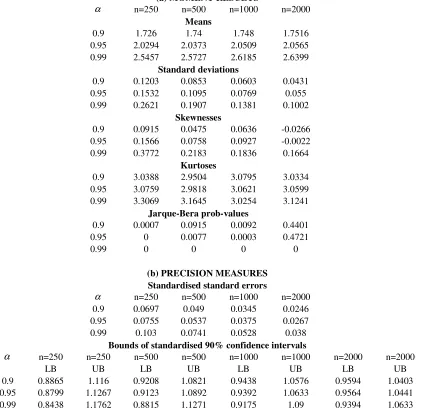
(a) MOMENT RESULTS
α n=250 n=500 n=1000 n=2000
Means
0.9 1.726 1.74 1.748 1.7516
0.95 2.0294 2.0373 2.0509 2.0565 0.99 2.5457 2.5727 2.6185 2.6399
Standard deviations
0.9 0.1203 0.0853 0.0603 0.0431 0.95 0.1532 0.1095 0.0769 0.055 0.99 0.2621 0.1907 0.1381 0.1002
Skewnesses
0.9 0.0915 0.0475 0.0636 -0.0266 0.95 0.1566 0.0758 0.0927 -0.0022 0.99 0.3772 0.2183 0.1836 0.1664
Kurtoses
0.9 3.0388 2.9504 3.0795 3.0334 0.95 3.0759 2.9818 3.0621 3.0599 0.99 3.3069 3.1645 3.0254 3.1241
Jarque-Bera prob-values
0.9 0.0007 0.0915 0.0092 0.4401
0.95 0 0.0077 0.0003 0.4721
0.99 0 0 0 0
(b) PRECISION MEASURES Standardised standard errors
α n=250 n=500 n=1000 n=2000
0.9 0.0697 0.049 0.0345 0.0246 0.95 0.0755 0.0537 0.0375 0.0267 0.99 0.103 0.0741 0.0528 0.038
Bounds of standardised 90% confidence intervals
α n=250 n=250 n=500 n=500 n=1000 n=1000 n=2000 n=2000
LB UB LB UB LB UB LB UB
0.9 0.8865 1.116 0.9208 1.0821 0.9438 1.0576 0.9594 1.0403 0.95 0.8799 1.1267 0.9123 1.0892 0.9392 1.0633 0.9564 1.0441 0.99 0.8438 1.1762 0.8815 1.1271 0.9175 1.09 0.9394 1.0633
TABLE 4: RESULTS FOR STANDARD NORMAL SPECTRAL RISK MEASURE
(a) MOMENT RESULTS
ARA n=250 n=500 n=1000 n=2000
Means
5 1.0863 1.0837 1.0831 1.0825 25 2.0326 1.9931 1.975 1.9647 100 2.9583 2.7264 2.6166 2.5597
Standard deviations
5 0.0836 0.0582 0.0411 0.0292
25 0.149 0.104 0.0719 0.0509
100 0.2823 0.1885 0.1264 0.088
Skewnesses
5 0.0226 0.0308 0.0379 -0.0338 25 0.1378 0.0577 0.0755 -0.0027 100 0.3099 0.1776 0.1573 0.1205
Kurtoses
5 2.958 2.9743 3.0832 3.0537
25 3.0654 2.9686 3.0575 3.0422 100 3.2012 3.1162 3.0388 3.0973
Jarque-Bera prob-values
5 0.4526 0.3946 0.0716 0.2113
25 0 0.051 0.0044 0.6854
100 0 0 0 0
(b) PRECISION MEASURES Standardised standard errors
ARA n=250 n=500 n=1000 n=2000
5 0.077 0.0537 0.0379 0.027
25 0.0733 0.0522 0.0364 0.0259 100 0.0954 0.0691 0.0483 0.0344
Bounds of standardised 90% confidence intervals
ARA n=250 n=250 n=500 n=500 n=1000 n=1000 n=2000 n=2000
LB UB LB UB LB UB LB UB
5 0.874 1.1263 0.9123 1.0901 0.9378 1.0633 0.9552 1.0443 25 0.8824 1.1243 0.9153 1.0869 0.9406 1.0609 0.9571 1.043 100 0.853 1.1628 0.8889 1.1182 0.9239 1.0821 0.9442 1.0577
Notes: Based on 10000 Monte Carlo simulation trials. ARA is the coefficient of absolute risk aversion,
TABLE 5: RESULTS FOR NORMAL VALUE AT RISK
Standardised standard errors
α n=250 n=500 n=1000 n=2000
N(0,1)
0.9 0.0857 0.0591 0.0426 0.0301 0.95 0.0817 0.0568 0.0403 0.0285 0.99 0.1003 0.071 0.0499 0.0356
N(5,1)
0.9 0.0173 0.012 0.0087 0.0061 0.95 0.0202 0.014 0.0099 0.0071 0.99 0.0318 0.0223 0.0158 0.0113
N(0,5)
0.9 0.0857 0.0591 0.0426 0.0301 0.95 0.0817 0.0568 0.0403 0.0285 0.99 0.1003 0.071 0.0499 0.0356
Bounds of standardised 90% confidence intervals
α n=250 n=250 n=500 n=500 n=1000 n=1000 n=2000 n=2000
LB UB LB UB LB UB LB UB
N(0,1)
0.9 0.8605 1.1447 0.9048 1.0991 0.9306 1.0707 0.9506 1.0494 0.95 0.8706 1.1367 0.9079 1.0964 0.9342 1.0679 0.9529 1.0466 0.99 0.8481 1.1747 0.8881 1.1236 0.921 1.0852 0.943 1.0601
N(5,1)
0.9 0.9718 1.0293 0.9807 1.0201 0.9859 1.0144 0.9899 1.0101 0.95 0.968 1.0338 0.9773 1.0237 0.9838 1.0168 0.9884 1.0115 0.99 0.9519 1.0553 0.9649 1.0388 0.9751 1.0269 0.9819 1.019
N(0,5)
0.9 0.8605 1.1447 0.9048 1.0991 0.9306 1.0707 0.9506 1.0494 0.95 0.8706 1.1367 0.9079 1.0964 0.9342 1.0679 0.9529 1.0466 0.99 0.8481 1.1747 0.8881 1.1236 0.921 1.0852 0.943 1.0601
TABLE 6: RESULTS FOR NORMAL EXPECTED SHORTFALL
Standardized standard errors
α n=250 N=500 n=1000 n=2000
N(0,1)
0.9 0.0697 0.049 0.0345 0.0246 0.95 0.0755 0.0537 0.0375 0.0267 0.99 0.103 0.0741 0.0528 0.038
N(5,1)
0.9 0.0179 0.0127 0.0089 0.0064 0.95 0.0218 0.0156 0.0109 0.0078 0.99 0.0347 0.0252 0.0181 0.0131
N(0,5)
0.9 0.0697 0.049 0.0345 0.0246 0.95 0.0755 0.0537 0.0375 0.0267 0.99 0.103 0.0741 0.0528 0.038
Bounds of standardised 90% confidence intervals
α n=250 n=250 n=500 N=500 n=1000 n=1000 n=2000 n=2000
LB UB LB UB LB UB LB UB
N(0,1)
0.9 0.8865 1.116 0.9208 1.0821 0.9438 1.0576 0.9594 1.0403 0.95 0.8799 1.1267 0.9123 1.0892 0.9392 1.0633 0.9564 1.0441 0.99 0.8438 1.1762 0.8815 1.1271 0.9175 1.09 0.9394 1.0633
N(5,1)
0.9 0.9709 1.0298 0.9796 1.0212 0.9855 1.0149 0.9895 1.0105 0.95 0.9653 1.0366 0.9746 1.0258 0.9823 1.0184 0.9873 1.0128 0.99 0.9473 1.0594 0.9598 1.0432 0.9716 1.0309 0.9791 1.0219
N(0,5)
0.9 0.8865 1.116 0.9208 1.0821 0.9438 1.0576 0.9594 1.0403 0.95 0.8799 1.1267 0.9123 1.0892 0.9392 1.0633 0.9564 1.0441 0.99 0.8438 1.1762 0.8815 1.1271 0.9175 1.09 0.9394 1.0633
TABLE 7: RESULTS FOR NORMAL SPECTRAL RISK MEASURE
Standardised standard errors
ARA n=250 n=500 n=1000 n=2000
N(0,1)
5 0.077 0.0537 0.0379 0.027
25 0.0733 0.0522 0.0364 0.0259 100 0.0954 0.0691 0.0483 0.0344
N(5,1)
5 0.0136 0.0095 0.0067 0.0048 25 0.0205 0.0146 0.0102 0.0073 100 0.0313 0.0229 0.0161 0.0115
N(0,5)
5 0.077 0.0537 0.0379 0.027
25 0.0733 0.0522 0.0364 0.0259 100 0.0954 0.0691 0.0483 0.0344
Bounds of standardised 90% confidence intervals
ARA n=250 n=250 n=500 n=500 n=1000 n=1000 n=2000 n=2000
0 LB UB LB UB LB UB LB UB
N(0,1)
5 0.874 1.1263 0.9123 1.0901 0.9378 1.0633 0.9552 1.0443 25 0.8824 1.1243 0.9153 1.0869 0.9406 1.0609 0.9571 1.043 100 0.853 1.1628 0.8889 1.1182 0.9239 1.0821 0.9442 1.0577
N(5,1)
5 0.9777 1.0224 0.9844 1.016 0.9889 1.0112 0.992 1.0079 25 0.9672 1.0347 0.9763 1.0243 0.9833 1.0171 0.988 1.0121 100 0.9518 1.0534 0.9632 1.0391 0.9747 1.0273 0.9814 1.0192
N(0,5)
5 0.874 1.1263 0.9123 1.0901 0.9378 1.0633 0.9552 1.0443 25 0.8824 1.1243 0.9153 1.0869 0.9406 1.0609 0.9571 1.043 100 0.853 1.1628 0.8889 1.1182 0.9239 1.0821 0.9442 1.0577
Notes: Based on 10000 Monte Carlo simulation trials. ARA is the coefficient of absolute risk aversion,
TABLE 8: RATIOS OF STATISTICS UNDER 2PN DISTRIBUTION TO THOSE UNDER STANDARD NORMAL DISTRIBUTION
VAR RISK MEASURE
Standardised standard errors
α n=250 n=500 n=1000 n=2000
0.9 1.130 1.162 1.134 1.140
0.95 1.120 1.134 1.127 1.137
0.99 1.106 1.087 1.092 1.110
Bounds of standardised 90% confidence intervals
α n=250 n=250 n=500 n=500 n=1000 n=1000 n=2000 n=2000
LB UB LB UB LB UB LB UB
0.9 0.981 1.012 0.986 1.014 0.988 1.011 0.997 1.009 0.95 0.980 1.015 0.988 1.008 0.992 1.009 0.995 1.007 0.99 0.981 1.019 0.991 1.006 0.991 1.007 0.995 1.004
ES RISK MEASURE
Standardized standard errors
α n=250 n=500 n=1000 n=2000
0.9 1.118 1.118 1.125 1.114
0.95 1.106 1.104 1.117 1.112
0.99 1.100 1.096 1.100 1.100
Bounds of standardized 90% confidence intervals
α n=250 n=250 n=500 n=500 n=1000 n=1000 n=2000 n=2000
LB UB LB UB LB UB LB UB
0.9 0.986 1.012 0.988 1.008 0.992 1.006 0.995 1.004 0.95 0.984 1.011 0.992 1.009 0.992 1.006 0.996 1.005 0.99 0.978 1.019 0.990 1.010 0.989 1.008 0.993 1.006
SRM RISK MEASURE
Standardised standard errors
ARA n=250 n=500 n=1000 n=2000
5 1.110 1.140 1.137 1.126
25 1.112 1.113 1.121 1.112
100 1.112 1.097 1.112 1.105
Bounds of standardised 90% confidence intervals
ARA n=250 n=250 n=500 n=500 n=1000 n=1000 n=2000 n=2000
LB UB LB UB LB UB LB UB
5 0.984 1.013 0.988 1.010 0.991 1.007 0.995 1.006 25 0.986 1.012 0.989 1.009 0.992 1.008 0.996 1.005 100 0.980 1.016 0.989 1.009 0.989 1.008 0.994 1.005
TABLE 9: RATIOS OF STATISTICS UNDER t DISTRIBUTION TO THOSE UNDER STANDARD NORMAL DISTRIBUTION
VAR RISK MEASURE
Standardised standard errors
α n=250 n=500 n=1000 n=2000
0.9 1.168 1.203 1.195 1.169
0.95 1.332 1.333 1.340 1.323
0.99 1.756 1.672 1.695 1.666
Bounds of standardised 90% confidence intervals
α n=250 n=250 n=500 n=500 n=1000 n=1000 n=2000 n=2000
LB UB LB UB LB UB LB UB
0.9 0.978 1.025 0.979 1.018 0.986 1.014 0.992 1.009 0.95 0.957 1.049 0.970 1.029 0.979 1.023 0.986 1.016 0.99 0.897 1.131 0.928 1.078 0.947 1.059 0.964 1.040
ES RISK MEASURE
Standardised standard errors
α n=250 n=500 n=1000 n=2000
0.9 1.515 1.533 1.522 1.537
0.95 1.722 1.698 1.715 1.730
0.99 2.199 2.157 2.186 2.232
Bounds of standardised 90% confidence intervals
α n=250 n=250 n=500 n=500 n=1000 n=1000 n=2000 n=2000
LB UB LB UB LB UB LB UB
0.9 0.948 1.062 0.958 1.044 0.972 1.030 0.981 1.022 0.95 0.925 1.094 0.944 1.064 0.959 1.043 0.971 1.034 0.99 0.852 1.201 0.886 1.146 0.910 1.101 0.932 1.081
SRM RISK MEASURE
Standardised standard errors
ARA n=250 n=500 n=1000 n=2000
5 1.344 1.348 1.335 1.333
25 1.850 1.831 1.832 1.853
100 2.273 2.285 2.302 2.369
Bounds of standardised 90% confidence intervals
ARA n=250 n=250 n=500 n=500 n=1000 n=1000 n=2000 n=2000
LB UB LB UB LB UB LB UB
5 0.962 1.050 0.969 1.029 0.979 1.021 0.986 1.015 25 0.915 1.105 0.935 1.073 0.954 1.051 0.968 1.037 100 0.858 1.200 0.891 1.144 0.913 1.106 0.935 1.080