What does a financial system say about future economic growth?

Munich Personal RePEc Archive

What does a financial system say about

future economic growth?

Grabowski, Szymon

Warsaw School of Economics

12 September 2008

Online at

https://mpra.ub.uni-muenchen.de/12834/

What does a financial system say about future

economic growth?

1

Szymon Grabowski

Warsaw School of Economics,

szymon.tomasz.grabowski@gmail.com

Abstract

In many research studies it is argued that it is possible to extract useful information about future economic growth from the performance of financial markets. However, this study goes further and shows that it is not only possible to use expectations derived from financial markets to forecast future economic growth, but that data about the financial system can be used for this purpose as well. The research is conducted for the Polish emerging economy on the basis of monthly data. The results suggest that, based purely on the data from the financial system, it is possible to construct reasonable measures that can, even for an emerging economy, effectively forecast future real economic activity. The outcomes are proved by two different econometric methods, namely, by a time series analysis and by a probit model. All presented models are tested in-sample and out-of-sample.

Key words: CCAPM, economic growth, financial markets, term spreads, expectations, fore-casting

JEL classification: G12, E43, E44

1

1

Introduction

In 1997 Harvey drew economists attention to variability of a yield curve and variability of real economic activity. In a simple framework of the CCAPM (the Consumption Based Capital Asset Pricing Model) he managed to explain why the shape of a yield curve can explain future real economic activity. Subsequently, many publications on this topic from various countries appeared. In 2007 Grabowski tested the possibility of forecasting real economic activity on the basis of the shape of a yield curve for the Polish economy. This paper is an extension of the previous research.

This time the author proves that the traditional leading indicators of real economic activity can be extended to other financial data variables. It is proposed to extend the list of potential predictors to a measure of financial stability and to stock market expectations towards the banking sector.

In the most common approaches, leading indicators of real economic activity are based on the real variables such as: number of housing permits, average weekly hours, average initial claims for unemployment insurance, etc. Recently, the list of potential variables has been extended to financial variables. For example in the USA, the New Jersey Index (see Orr et al. (2001)) comprises of yield spreads which are used to forecast nine-month economic growth in New Jersey and in the New York State. Economists often include stock market expectations in leading indicators. However, the list seems not to be limited. In this paper, the author presents that a measure of financial stability as well as stock market expectations toward the banking sector can be utilised to improve performance of the leading indicators of economic activity.

The article is different from its counterparts, since it presents research conducted for an emerging economy. A standard time series analysis is extended with a probit model specifi-cation. The author tests the forecasting ability of the proposed models in-sample and out-of-sample.

2

Economic rationale

2.1

Established leading indicators

Originally, leading indicators were introduced to forecast real economic activity. The first types of leading indicators were mainly based on the idea that some segments of the economy might react faster to changes in the business cycle. For example it is assumed that an increase in average initial claims for unemployment insurance might lead economic contraction. Later economists started to include information coming from the financial system. Very often agents’ expectations were included by adding variables such as returns on stock market or yield spreads calculated for instruments of a different maturity. Based on this, economists suggested various explanations for expectations to forecast real economic activity. The article of Harvey (1997) proposes the CCAPM framework to explain future economic activity. A similar economic rationale was presented in Brock (1982)(but for the supply side of the economy).

Other researchers such as Pena and Rodriguez (2006) proposes a framework in which agents’ expectations might be derived from the stock market as well as from the shape of a yield curve. In this way the authors used both expectations extracted from the stock market and from the term structure of interest rates to forecast real economic activity. This paper sheds light on the ability to forecast real economic activity, based on additional and different financial variables than what have been presented so far.

2.2

Newly proposed leading indicators

The idea to use additional financial data to forecast real economic activity is based on two notions. On the one hand, the author believes that a financial system can be perceived as an indicator of investors’ expectations. On the other hand, shocks that have a root in a financial system might easily transmit to the real economy. In this paper the first notion is presented by stock market expectations toward the banking sector. The second notion is introduced by a simple proxy of financial stability.

2.2.1 Stock market expectations – the banking sector

There is a vast literature that presents the usefulness of stock market indicators in predicting real economic activity. This study also refers to this stream of the literature.

A positive relation between the banking sector and real economic activity is presented in a wide spectrum of research. An interesting approach to this issue is presented in Cole, Moshirian, and Wu (2007), in which the authors concluded that the positive relation between real economic activity and excess stock market returns exists in all examined countries. The approach presented in this paper is quite different. Instead of using excess stock market returns, the relative stock market returns in relation to general stock market returns are used. The relation depicting expectations toward the banking sector is presented by equation 1.

ex bankt =log(

W IG bankit

W IG bankit−12

)₋log( W IGt

W IGt−12

) (1)

where:

W IG is the Warsaw Stock Market Index,

W IG banks is the Warsaw Stock Market Index for banks listed on the stock market exchange.

The proposed approach has one more advantage. The presentation of an expected condition of the banking sector in relation to a general stock market index solves the problem of a general stock market bubble. Relation 1 measures how the banking sector is perceived by investors in relation to the whole market. If stock market returns concerning the banking sector are higher than returns in the other sectors, investors assessment of future performance of the banks are also more profitable.

Future performance of the banking sector might be useful in predicting real economic activity due to the structure of profits of the Polish banking sector. The majority of banks’ profits constitute of an interest profit which is reliant on credit growth. In 2007 more than 50% of profits of the Polish banking sector comprised of interest income. Credits are granted to the real sector as mortgages, consumer credits or investment credits, which in turn (as presented in Bernanke et al. (1998)) accelerate the consumption and investments, and in this way increase the real economic activity.

The predictability of stock market expectations toward the banking sector might be closely connected with the credit channel. To this end, Wrobel et al. (2008) prove that the credit channel exists in Poland.

2.2.2 Financial Stability

market in Poland has been changing the structure of the financial system. Gradually, financial markets are becoming more crucial for stable growth in Poland. However, from the beginning of the nineties the banking sector has played the most important role in the financing of the real economy.

As far as the banking sector and forecasting real economic activity are concerned, it is robustness of banks that seems to have an important impact on the real economy. To finance the real economy, banks need to acquire capital. On the one hand, credits granted by banks are very often given for a relatively long period of time. One the other hand, the financial sources acquired by banks are short-term liabilities that need to be renewed on a short-term basis (some times even on a monthly or weekly basis). Due to the fact that banks are a key intermediary, redistributing financial sources in the Polish economy, it is very important to monitor the risk contained in the banking sector. As the recent banking crises showed, the banking system’s instability easily transforms into a credit crunch that slows down the real economy. As a result, access to financial sources needed, for investments and reconstructions of companies are constrained.

Usually an increasing risk in the banking sector could be visible in increasing risk premium. It is the result of banks’ reluctance to lend financial sources to institutions perceived as more risky. In such cases, financial institutions are willing to lend but they require higher margins.

Moreover, if a risky institution is important for the whole system (important from the systemic point of view) all banks will increase margins, rising risk premium in the banking system as a whole in this way. As a result, financing becomes more expensive and constrains credits granted to the non-financial sector of the economy. The costs of lending among banks might be well measured by the money market interest rates. Monitoring a spread between short term money market interest rates and the reference rate of the Central Bank indicates the level of credit risk of financial institutions. Consequently, in the empirical part of the article the risk premium observed on the interbank market is depicted by the following variable:

Riskt=R BCt−R M arkett (2)

where:

R BC is the reference rate of Central Bank,

R M arketis the monthly average of Wibor(1M)2

.

2

3

Empirical Analysis

3.1

Time series analysis

The basic economic framework for the empirical analysis of this section is presented in, Harvey (1997), Ferreira et al. (2003), Pena and Rodriguez (2006). A special focus on Poland is proposed in Grabowski (2007). The basic CCAPM and PCAPM specifications are extended to a proxy of risk of a financial system and stock market expectations concerning the banking sector. To test robustness of the results, the relation is tested for the supply and demand side of the economy. As in Grabowski (2007) measures of real economic activity are real retail sale ∆rrst,t−k (demand) and real industrial production ∆rspt,t−k (supply).

The empirical verification of the relation between real economic activity and the financial system is based on the economic rationale presented in section 2. The basic economic framework is the CCAPM proposed by Harvey (1997) in which yield spreads are lagged at least 12 periods. To keep the whole analysis in line with the CCAPM all remaining explanatory variables are also lagged at least 12 periods. The variable Risk, describing distress in a financial system, is lagged 12 periods because it is assumed that some shocks transmit to the real economy with a lag ,but not necessarily longer than one year. Only N Y St−p−1,1,2 is lagged 13 periods which is

in line with the CCAPM model presented in Harvey (1997). The variable N Y St−p−1,1,2 is the

spread between yields of 2-year Polish government bonds and yields of one-year treasury bills. As presented in Grabowski (2007) this is the only yield spread that is stationary and do not disagree with the economic framework presented in Harvey (1997).

As far as equity market expectations are concerned, it is believed that the stock market prices contain information on future performance of the company. In every point in time investors present their n-period expectations toward performance of the particular company. In this way the relation 1 is the difference between n-period investors’ expectations for the banking sector versus their expectations for the remaining sectors of the economy listed on a stock market. Assuming that the horizon of these expectations is at least 12 periods the variable ex bank

ought to be lagged at least 12 periods. In this way the varying relative expectations will match with ex-post one year economic activity.

Due to the lack of a perfect measure of real economic activity, the robustness of outcomes is tested for the supply and demand sides of the economy. The detailed construction of the data is presented in appendix. The equations for the demand side (eq. 3) and supply side (eq. 4) of the economy are presented below:

∆rrst,t−k=α+β1N Y St−p−1,1,2+β2Riskt−p +β3ex bankt−p

∆rspt,t−k =α+β1N Y St−p−1,1,2+β2Riskt−p+β3ex bankt−p

+γ1D2005:04+γ2D2004:04+γ3D2005:02

+γ4D2005:03+γ5D2004:03+γ6D2004:02+µt−k (4)

Both specifications include dummy variables because the effects of EU accession ought to be eliminated from the time series in order not to blur the final results. The model specification explaining the supply side of the economy involves more dummy variables since it is assumed that production side of the economy need more time to adjust to the institutional changes than the demand side of the economy.

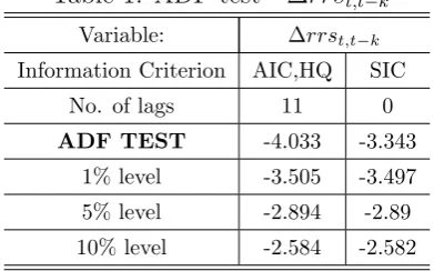
Time series are tested for unit-root. The results are given in the tables from 1 to 8. Table 1: ADF test - ∆rrst,t−k

Variable: ∆rrst,t₋k

Information Criterion AIC,HQ SIC No. of lags 11 0

ADF TEST -4.033 -3.343

1% level -3.505 -3.497 5% level -2.894 -2.89 10% level -2.584 -2.582

Table 2: KPSS test - ∆rrst,t−k Variable: ∆rrst,t₋k

Information Criterion

Newey-West Bartlett kernel

Andrews Bartlett kernel

Newey-West Parzen kernel

Andrews Parzen kernel

Bandwidth 8 14.5 13 29.5

KPSS test 0.171 0.132 0.152 0.12

1% level 0.739 0.739 0.739 0.739 5% level 0.463 0.463 0.463 0.463 10% level 0.347 0.347 0.347 0.347

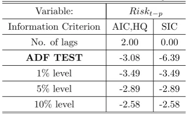
The figures in tables suggest that all variables are stationary in mean and parameters in equations 3 and 4 may be estimated without a thread of spurious regression.

Two models passed the test for collineraity and the Jarque-Bera test for normal distribution of residuals. Since in all estimated models the autocorrelation is present, the t-Statistic from an ordinary least squares regression will be incorrect.3

The Newey and West (1987) technique

3

Table 3: ADF test ∆rspt,t−k Variable: ∆rspt,t₋k

Information Criterion AIC,HQ SIC No. of lags 1 0

ADF TEST -2.782 -4.559

1% level -3.495 -3.495 5% level -2.890 -2.889 10% level -2.582 -2.581

Table 4: KPSS test - ∆rspt,t−k Variable: ∆rspt,t₋k

Information Criterion Newey-West Bartlett kernel Andrews Bartlett kernel Newey-West Parzen kernel Andrews Parzen kernel

Bandwidth 8 9.46 13 17.8

KPSS test 0.397 0.363 0.353 0.303

1% level 0.739 0.739 0.739 0.739 5% level 0.463 0.463 0.463 0.463 10% level 0.347 0.347 0.347 0.347

Table 5: ADF test - Riskt−p Variable: Riskt₋p

Information Criterion AIC,HQ SIC No. of lags 2.00 0.00

ADF TEST -3.08 -6.39

1% level -3.49 -3.49 5% level -2.89 -2.89 10% level -2.58 -2.58

Table 6: KPSS test - Riskt−p

Variable: Riskt₋p

Information Criterion Newey-West Bartlett kernel Andrews Bartlett kernel Newey-West Parzen kernel Andrews Parzen kernel Bandwidth 10.00 5.14 12.00 9.21

KPSS test 0.568 0.936 0.626 0.792

Table 7: ADF test - Ex bankit−p Variable: Ex bankit₋p

Information Criterion AIC,HQ SIC No. of lags 11.00 1.00

ADF TEST -2.623 -1.845

1% level -3.512 -3.503 5% level -2.897 -2.893 10% level -2.585 -2.583

Table 8: KPSS test -Ex bankit−p Variable: Ex bankit₋p

Information Criterion

Newey-West Bartlett kernel

Andrews Bartlett kernel

Newey-West Parzen kernel

Andrews Parzen kernel Bandwidth 7.00 48.9 11,00 128

KPSS test 0.225 0.265 0.203 0.618

1% level 0.739 0.739 0.739 0.739 5% level 0.463 0.463 0.463 0.463 10% level 0.347 0.347 0.347 0.347

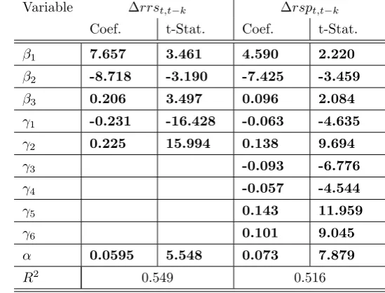
Table 9: The estimates on the sample: 2000:05 2007:07 - yield spreads lagged 12 periods

Variable ∆rrst,t₋k ∆rspt,t₋k

Coef. t-Stat. Coef. t-Stat.

β1 7.657 3.461 4.590 2.220

β2 -8.718 -3.190 -7.425 -3.459

β3 0.206 3.497 0.096 2.084

γ1 -0.231 -16.428 -0.063 -4.635

γ2 0.225 15.994 0.138 9.694

γ3 -0.093 -6.776

γ4 -0.057 -4.544

γ5 0.143 11.959

γ6 0.101 9.045

α 0.0595 5.548 0.073 7.879

R2

is used to recalculate the t-Statistic. The bold lines mean statistical significance at least at the level of 5%.

The results are in-line with the economic rational presented in section 2 and have the same interpretation in both models. The decreasing value of theN Y S(positive parameterβ1) implies that the yield curve inverts. An inverted yield curve might, inter alia, suggest that a level of a long-term savings in debt instruments increases and consumption decreases. A reduction in the consumption level constrains the internal demand and slows the economy.

The negative sign in front of β2 also confirms economic theory. The increasing spread between the reference rate and money market rate implies growing credit risk concealed in the banking sector. As a result, banks are reluctant to lend money to each other and will probably constrain the number of granted credits to the real sector. The serious financing problems present in the banking sector very often lead to a credit crunch. Assuming that the effective credit channel is present in the economy the constrained lending should slow the economy.

In very extreme cases, the tensions present in the financial system lead to financial crises. In this sense the financial disturbances can be very expensive for the whole economy. A detailed costs analyses of banking crises are presented in Klingebiel, Kroszner, and Laeven (2004).

The last structural parameter β3 presents how investors perceive the profitability of the banking sector. In a banking-based financial system this perception might be a proxy for an increase in future credit. It is the interest income that is the most important and stable part of banks’ income. In Poland more than 50% of the banks’ profit comprise of interest income. Investors that expect better performance of the banking sector might indirectly forecast future credit expansion.

In banking oriented economies, banks supply the economy with the essential sources for investments and for the financing of current operations. The positive sign in both equations 3 and 4 means that investors expect that banks will perform better than other sectors of the economy, implying indirectly credit expansion which will probably accelerate the economy.

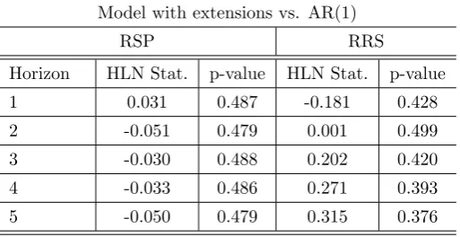
In-sample performance of the model is acknowledged by the out-of-sample statistics. The table 10 and 11 present the version of Diebold-Mariano statistic for small sample as presented in Harvey, Leybourne, and Newbold (1997).

Table 10 presents how forecasts of the model with a proxy of financial stability and stock market expectations toward the banking sector differ from forecasts of the model based only on the CCAPM (PCAPM) rationale. The figures in the table 11 compare the forecasts accuracy of models 3 and 4 with AR(1) models 4

.

The presented test results are calculated starting from the sample size of 50 observations5

.

4

The number of lags was selected on the basis of BIC information criterion. The tests were also conducted for lags of 3 as selected by AIC information criterion but the conclusions were the same.

5

Table 10: Models’ forecast performance comparison

Models with extensions vs. basic model (yield spreads)

RSP RRS

Horizon HLN Stat. p-value HLN Stat. p-value 1 -1.585 0.062 -2.260 0.016 2 -1.531 0.066 -2.027 0.024 3 -1.621 0.055 -2.023 0.023 4 -1.687 0.047 -2.113 0.018 5 1.811 0.036 -2.173 0.015

Table 11: Models’ forecast performance comparison

Model with extensions vs. AR(1)

RSP RRS

Horizon HLN Stat. p-value HLN Stat. p-value 1 0.031 0.487 -0.181 0.428 2 -0.051 0.479 0.001 0.499 3 -0.030 0.488 0.202 0.420 4 -0.033 0.486 0.271 0.393 5 -0.050 0.479 0.315 0.376

The models are recursively estimated and forecasts of the horizon of 1, 2, 3, 4, 5 periods are generated. Next, the errors of forecasts are calculated for every horizon of forecast and Diebold-Mariano statistic is calculated. The presented results take the adjustment of the DM statistic into account for the small samples as presented in Harvey, Leybourne, and Newbold (1997).

In the paper of Clark and McCracken (1999) the authors suggest that if forecasting models are nested many of the usual test statistics fail to converge to the standard normal distribution. This implies that the results presented in the table 10 might be misleading. However, using statistics proposed in Clark and McCracken (1999) give the same conclusions.

3.2

Probit model

This section refers to the publication of Estrella and Trubin (2006) in which the probit model is used to forecast periods of recession in the United States. It is another way of testing the usefulness of the financial variables in forecasting real economic activity. It might be interpreted as a complimentary approach due to the fact that a different econometric method is implemented.

A standard probit model specification presented in Estrella and Trubin (2006) is extended with additional explanatory variables. It also offers construction of a probability model for an

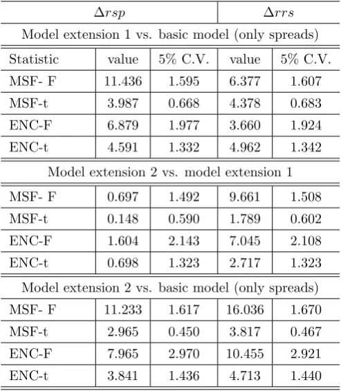
Table 12: Models’ forecast performance comparison (1-step horizon)

∆rsp ∆rrs

Model extension 1 vs. basic model (only spreads)

Statistic value 5% C.V. value 5% C.V. MSF- F 11.436 1.595 6.377 1.607 MSF-t 3.987 0.668 4.378 0.683 ENC-F 6.879 1.977 3.660 1.924 ENC-t 4.591 1.332 4.962 1.342

Model extension 2 vs. model extension 1

MSF- F 0.697 1.492 9.661 1.508 MSF-t 0.148 0.590 1.789 0.602 ENC-F 1.604 2.143 7.045 2.108 ENC-t 0.698 1.323 2.717 1.323

Model extension 2 vs. basic model (only spreads) MSF- F 11.233 1.617 16.036 1.670 MSF-t 2.965 0.450 3.817 0.467 ENC-F 7.965 2.970 10.455 2.921 ENC-t 3.841 1.436 4.713 1.440

emerging market.

The construction of probability models for emerging markets is a challenging task. The first obstacle that occurs is the lack of the reference variable. Unfortunately there is no equivalent of the National Bureau of Economic Research that specifies exact and unambiguous dates of recessions and economic expansions.

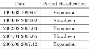
The author finds the values of the reference variable by referring to different publications concerning business cycles in Poland and by estimating M S₋AR on time series of real retail sale (rrs) and real sold production (rsp) in the industry. The dates suggested by MS-AR are compared with dates from economic publications and appropriate adjustments are made. The methodology of extracting the reference variable of an economic slowdown is complex enough to be described in a separate paper and will thus not be presented here.

Table 13: The reference variable – period classification

Date Period classification

1999:03 1999:07 Expansion 1999:08 2002:02 Slowdown 2002:02 2004:03 Expansion 2004:04 2005:05 Slowdown 2005:06 2007:12 Expansion

thought difficult to forecast ex-ante. Nevertheless, the probability model based on the financial indicators could forecast even such extreme cases.

Model specification is quite similar to eq. 3 or eq. 4. The difference is that there is no dummy variables in periods concerning pre-accession and after accession periods. As the model is a probability model of economic slowdown, fitted values ought to vary between 0 and 1. This is guaranteed by the probit model specification:

Zt=α+β1N Y St−p−1,1,2+β2Riskt−p+β3ex bankt−p+ǫt (5)

Assuming as in Estrella and Trubin (2006) that the ǫt follows the normal distribution the

probit model can be written as:

P(yt= 1) =F(Zt) = Z Zt

∞

1

√

2πe −t2

2 dt (6)

The variableZtin 6 is latent, not observable, variable depicting the probability of the Polish

economy to fall into economic slowdown. TheZtis defined as in 7 and is the ”observable” binary

variable discriminating between periods of economic expansion and economic slowdown:

yt=  



1 if Zt>0

0 otherwise

(7) Model is estimated by ML method and the results are as presented in the table 14:

Table 14: The probit model estimates on the sample: 2000:05 2007:07

Variable Yt

Coef. Z-Stat.

β1 -1045.630 -2.137

β2 1594.647 1.948

β3 -80.488 -2.067

α -6.735 -1.932

M cF addenR2

0.895

an economic slowdown decreases as the value of the yield spread increases and the probability of an economic slowdown decreases as the excess return on equities of the banking sector increases. The increasing value of the banking sector risk indicator increases the probability of the slowdown.

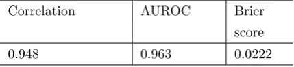
The in-sample performance of the model seems to be satisfied, however how well the model forecasts can be tested in out-of-sample tests. Figure 1 shows how well the model identifies the periods of economic slowdown in Poland. The model discriminates properly between periods of economic expansion and economic slowdown in 96.43%.

Figure 1: Fitted versus actual values

0.0 0.2 0.4 0.6 0.8 1.0

0.0 0.2 0.4 0.6 0.8 1.0

2001 2002 2003 2004 2005 2006 2007

Actual Fitted

Table 15: The forecast performance tests

Correlation AUROC Brier score

0.948 0.963 0.0222

4

Conclusions

The overall conclusion is that it is possible to build leading indicators on the basis of financial variables. Grabowski (2007) and Mehl (2006) show that the forecasting ability of an inverting yield curve can be applied also to an emerging market economy. This study goes further and presents that an extension of the models, based on the CCAPM or PCAPM rationale with other reasonable ”financial” variables, gives the possibility to forecast real economic activity in Poland.

The explanatory variables are selected on the basis of economic rationale. The first one depicts how investors perceive the profitability of the banking sector in relation to other sectors of the economy listed on the stock market. Since more than 50% of the income of the Polish banking sector comes from the interest income it might be possible that investors indirectly forecast credit expansion. Moreover, as many papers present a robust financial system is needed for sustained economic growth and effective monetary policy.

The second explanatory variable is a proxy of the tension in the financial system. The course of the financial crises shows that turmoil in the financial system usually results in a credit crunch and an economic slowdown.

Robustness of the results is confirmed by different econometric methods. On the one hand, the satisfactory in-sample results are confirmed by out-of-sample tests. On the other hand, the methodology suggested by Estrella and Trubin (2006) gives astonishingly good results that are coherent with conclusions from standard time series analysis.

References

Andrews, D., 1991. Heteroskedasticity and autocorrelation consistent covariance matrix esti-mation. Econometrica 59 (3).

Bernanke, B., Gertler, M., Gilchrist, S., 1998. The financial accelerator in a quantitative busi-ness cycle framework. NBER Working Papers 6455, National Bureau of Economic Research, Inc.

Brock, W. A., 1982. Asset pricing in a production economy. Tech. rep., The Economics of Uncertainty and Information, University of Chicago Press.

Clark, T. E., McCracken, M. W., 1999. Tests of equal forecast accuracy and encompassing for nested models. Tech. rep.

Cole, R., Moshirian, F., Wu, Q., 2007. Bank stock returns and economic growth. Mpra paper, University Library of Munich, Germany.

Estrella, A., Trubin, M. R., 2006. The yield curve as a leading indicator: some practical issues. In: Current Issues in Economics and Finance. Vol. 12. Federal Reserve Bank of New York. Ferreira, E., Martinez, M. I., Navarro, E., Rubio, G., 2003. Real activity and

yield spreads under the consumption-based asset pricing model, storna internetowa: http://www.ucm.es/info/icae/seminario/seminario0304/07oct.pdf.

Grabowski, S., 2007. Real economic activity and state of financial markets. In: Department of Applied Econometrics Working Papers – Warsaw School of Economics. No. 7-07.

Harvey, C. R., 1997. The relation between the term structure of interest rates and Canadian economic growth. Canadian Journal of Economics.

Harvey, D., Leybourne, S., Newbold, P., 1997. Testing the equality of prediction mean squared errors. International Journal of Forecasting 13.

Klingebiel, D., Kroszner, R., Laeven, L., 2004. Financial crises, financial dependence and in-dustrial growth. Policy research working paper series, The World Bank.

Mehl, A., 2006. The yield curve as predictor and emerging economies. In: European Central Bank Working Papers Series. No. 691.

Newey, W., West, K., 1995. Automatic lag selection in covariance matrix estimation. NBER Technical Working Papers 0144, National Bureau of Economic Research, Inc.

Orr, J., Rich, R., Rosen, R., 2001. Leading economic indexes for New York state and New Jersey. FRBNY Economic Policy Review.

Pena, J. I., Rodriguez, R., 2006. On the economic link between asset prices and real activity. Business Economic Series of Universidad Carlos III de Madrid.

APPENDIX

DATA DESCRIPTION

∆rsst,t−k=ln

rsst

rsst−k

(A-1)

rsst - denotes real seasonally adjusted level of retail sale, monthly data, source Polish Central

Statistical Office.

∆rspt,t−k=ln

rspt

rspt−k

(A-2)

rspt- denotes real seasonally adjusted level of industrial production,monthly data, source Polish

Central Statistical Office.

In the presented article one year logarithmic increments of rss and rsp are used (k = 12, ∆rsst,t−12 and ∆rspt,t−12 ).

N Y St−p−1,t,t+N =

1 +Rt+N

1 +Rt (A-3)

N Y St−p−1,t,t+N - denotes nominal bond yield spread lagged p−1 months

Rt+N _{- denotes nominal yield of Polish government benchmark bond maturing in N years (long}

interest rate), monthly data, period average, source Reuters

Rt _{- denotes yield of Polish treasury bills (short interest rate): 3-month treasury bills or}

12-month treasury bills, 12-monthly data, period average,source Polish Ministry of Finance The seasonally adjusted time series are derived by means of TramoSeats procedure.

EXAMPLES OF DATA ENCODING

N Y St−12,0.25,3 - denotes 12-month lagged nominal yield spread calculated between yield of

3-month (13-week) treasury bills and yield of Polish benchmark bonds maturing in 3 years

N Y St−13,1,2 - denotes 13-month lagged nominal yield spread calculated between yield of 1-year

(52-week) treasury bills and yield of Polish benchmark bonds maturing in 2 years

UNIT ROOT TESTS

Table A-1: Philips Perron test for rsp

Variable: rsp

Information Criterion Newey-West-Bartlett kernel Andrews Bartlett kernel Newey West Parzen kernel Andrews Parzen kernel

Bandwidth 5 3.71 10 4.33

Phillips-Perron test -4.627 -4.531 -4.876 -4.255

1% level -3.495 -3.495 -3.495 -3.495

5% level -2.889 -2.889 -2.889 -2.889

10% level -2.581 -2.581 -2.581 -2.581

Table A-2: Phillips-Perron test for rrs

Variable: rrs

Information Criterion Newey-West-Bartlett kernel Andrews Bartlett kernel Newey West Parzen kernel Andrews Parzen kernel

Bandwidth 6 2.31 14 3.62

Phillips-Perron test -3.213 -2.982 -3.398 -2.956

1% level -3.497 -3.497 -3.497 -3.497

5% level -2.891 -2.891 -2.891 -2.891

10% level -2.582 -2.582 -2.582 -2.582

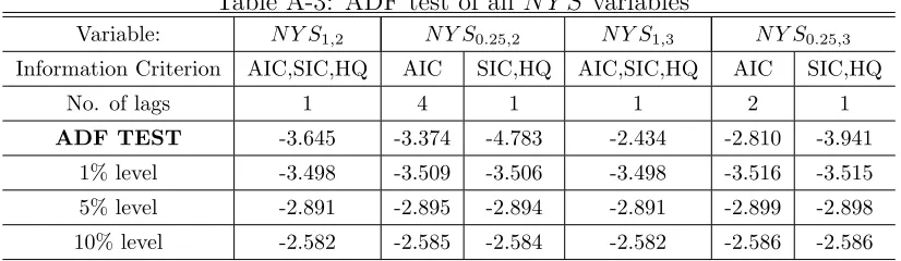
Table A-3: ADF test of all N Y S variables

Variable: N Y S1,2 N Y S0.25,2 N Y S1,3 N Y S0.25,3

Information Criterion AIC,SIC,HQ AIC SIC,HQ AIC,SIC,HQ AIC SIC,HQ

No. of lags 1 4 1 1 2 1

ADF TEST -3.645 -3.374 -4.783 -2.434 -2.810 -3.941

1% level -3.498 -3.509 -3.506 -3.498 -3.516 -3.515 5% level -2.891 -2.895 -2.894 -2.891 -2.899 -2.898 10% level -2.582 -2.585 -2.584 -2.582 -2.586 -2.586

Table A-4: Phillips-Perron test of N Y S1,2

Variable: N Y S1,2

Information Criterion Newey-West Bartlett kernel Andrews Bartlett kernel Newey West Parzen kernel Andrews Parzen kernel

Bandwidth 3 3.36 9 6.17

Phillips-Perron test -3.238 -3.227 -2.989 -3.192

1% level -3.497 -3.497 -3.497 -3.497

5% level -2.891 -2.891 -2.891 -2.891

10% level -2.582 -2.582 -2.582 -2.582

Table A-5: KPSS test ofN Y S1,2

Variable: N Y S1,2

Information Criterion Newey-West-Bartlett kernel Andrews Bartlett kernel Newey West Parzen kernel Andrews Parzen kernel

Bandwidth 11 17.1 12 36

KPSS test 0.671 0.555 0.772 0.414

1% level 0.739 0.739 0.739 0.739

5% level 0.463 0.463 0.463 0.463

10% level 0.347 0.347 0.347 0.347

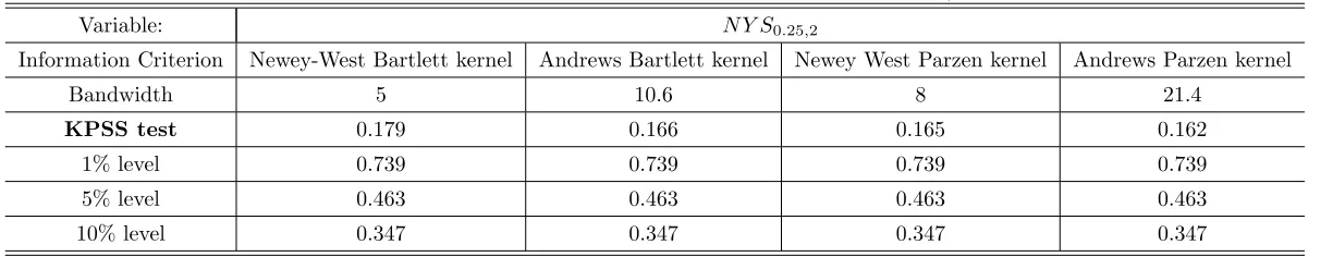
Table A-6: KPSS test of N Y S0.25,2

Variable: N Y S0.25,2

Information Criterion Newey-West Bartlett kernel Andrews Bartlett kernel Newey West Parzen kernel Andrews Parzen kernel

Bandwidth 5 10.6 8 21.4

KPSS test 0.179 0.166 0.165 0.162

1% level 0.739 0.739 0.739 0.739

5% level 0.463 0.463 0.463 0.463

10% level 0.347 0.347 0.347 0.347

Table A-7: Phillips-Perron test of N Y S0.25,2

Variable: N Y S0.25,2

Information Criterion Newey-West-Bartlett kernel Andrews Bartlett kernel Newey West Parzen kernel Andrews Parzen kernel

Bandwidth 6 3.37 11 6.3

Phillips-Perron test -3.531 -3.681 -3.420 -3.680

1% level -3.514 -3.514 -3.514 -3.514

5% level -2.898 -2.898 -2.898 -2.898

10% level -2.586 -2.586 -2.586 -2.586

Table A-8: KPSS test ofN Y S1,3

Variable: N Y S1,3

Information Criterion Newey-West Bartlett kernel Andrews Bartlett kernel Newey West Parzen kernel Andrews Parzen kernel

Bandwidth 8 33.9 13 81.7

KPSS test 0.972 0.384 0.845 0.329

1% level 0.739 0.739 0.739 0.739

5% level 0.463 0.463 0.463 0.463

10% level 0.347 0.347 0.347 0.347

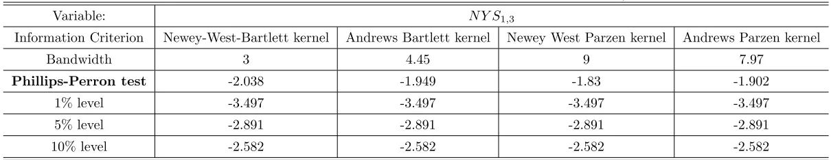
Table A-9: Phillips-Perron test of N Y S1,3

Variable: N Y S1,3

Information Criterion Newey-West-Bartlett kernel Andrews Bartlett kernel Newey West Parzen kernel Andrews Parzen kernel

Bandwidth 3 4.45 9 7.97

Phillips-Perron test -2.038 -1.949 -1.83 -1.902

1% level -3.497 -3.497 -3.497 -3.497

5% level -2.891 -2.891 -2.891 -2.891

10% level -2.582 -2.582 -2.582 -2.582

Table A-10: KPSS test of N Y S0.25,3

Variable: N Y S0.25,3

Information Criterion Newey-West Bartlett kernel Andrews Bartlett kernel Newey West Parzen kernel Andrews Parzen kernel

Bandwidth 6 14.3 9 30.4

KPSS test 0.683 0.521 0.699 0.387

1% level 0.739 0.739 0.739 0.739

5% level 0.463 0.463 0.463 0.463

10% level 0.347 0.347 0.347 0.347

Table A-11: Phillips-Perron test of N Y S0.25,3

Variable: N Y S0.25,3

Information Criterion Newey-West-Bartlett kernel Andrews Bartlett kernel Newey West Parzen kernel Andrews Parzen kernel

Bandwidth 6 3.76 11 6.98

Phillips-Perron test -2.839 -3 -2.715 -2.971

1% level -3.514 -3.514 -3.514 -3.514

5% level -2.898 -2.898 -2.898 -2.898

10% level -2.586 -2.586 -2.586 -2.586

Table A-12: Phillips-Perron test forRisk

Variable: Risk

Information Criterion Newey-West-Bartlett kernel Andrews Bartlett kernel Newey West Parzen kernel Andrews Parzen kernel

Bandwidth 5.00 1.88 9.00 3.29

Phillips-Perron test -6.847 -6.216 -7.051 -6.342

1% level -3.498 -3.498 -3.498 -3.498

5% level -2.891 -2.891 -2.891 -2.891

10% level -2.582 -2.582 -2.582 -2.582

Table A-13: Phillips-Perron test for Ex bank

Variable: Ex bank

Information Criterion Newey-West-Bartlett kernel Andrews Bartlett kernel Newey West Parzen kernel Andrews Parzen kernel

Bandwidth 4.00 4.61 8.0 8.33

Phillips-Perron test -1.664 -1.683 -1.759 -1.769

1% level -3.502 -3.502 -3.502 -3.502

5% level -2.892 -2.892 -2.892 -2.892

10% level -2.583 -2.583 -2.583 -2.583