http://dx.doi.org/10.4236/tel.2014.42022
How to cite this paper: Matsumoto, A. and Szidarovszky, F. (2014) Dynamic Monopoly with Demand Delay. Theoretical Economics Letters, 4, 146-154. http://dx.doi.org/10.4236/tel.2014.42022
Dynamic Monopoly with Demand Delay
Akio Matsumoto1, Ferenc Szidarovszky2
1Department of Economics, Chuo University, Tokyo, Japan
2Department of Applied Mathematics, University of Pécs, Pécs, Hungary Email: [email protected], [email protected]
Received 26 December 2013; revised 26 January 2014; accepted 2 February 2014
Copyright © 2014 by authors and Scientific Research Publishing Inc.
This work is licensed under the Creative Commons Attribution International License (CC BY).
http://creativecommons.org/licenses/by/4.0/
Abstract
This study analyses the dynamics of nonlinear monopoly. To this end, the conventional assump-tions in the text-book monopoly are modified; first, the complete information on the market is re-placed with the partial information; second, the instantaneous information is substituted by the delay information. As a result, since such a monopoly is unable to jump, with one shot, to the op-timal point for which the profit is maximized, the monopoly has to search for it. In a continuous- time framework, the delay destabilizes the otherwise stable monopoly model and generates cyclic oscillations via a Hopf bifurcation. In a discrete-time framework, the steady state bifurcates to a bounded oscillation via a Neimark-Sacker bifurcation. Although this has been only an introduction of delay into the traditional monopoly model, it is clear that the delay can be a source of essential-ly different behavior from those of the nondelay model.
Keywords
Monopolist Competition; Demand Fluctuations; Bounded Rationality; Fixed Time Delay; Continuous and Discrete Dynamics
1. Introduction
147
jump to the optimal point but searches for it with using the actual data obtained through the market. The mod-ified model becomes dynamic in nature. This is the issue far outside the scope of the text book monopoly and it is what we will consider in this study.
In the recent literature, various learning processes of the boundedly rational monopolist have been extensively studied. Puu [1] constructs a discrete-time monopoly model in which price function is cubic and cost function is linear. It is shown that the gradient learning or search process based on locally obtained information might be-have in an erratic way under the condition that the price function has an inflection point. Assuming that the mo-nopolist uses a rule of thumb to determine quantity to produce, Naimzada and Ricchiuti [2] reconsider Puu’s model with a linear cost function and a cubic price function without the inflection point. Their model is then ge-neralized by Asker [3] who replaces the cubic function with higher-order polynomials. Matsumoto and Szida-rovszky [4] further generalize Asker’s model by introducing the more general type of the cost function. Since those models are described by one dimensional difference equation, chaotic dynamics can arise via pe-riod-doubling bifurcation.
In this study we reconsider a dynamic monopoly model from two different points of view. First, to detect the effect caused by non-instantaneous information, the dynamic process is constructed in continuous-time scales and a fixed time delay is introduced. Second, we discretize the continuous process to obtain a “delay” discrete process and analyze the delay effect on discrete dynamics. In both models, local stability of a stationary state is analytically considered and global dynamics is numerically examined.
The paper is organized as follows. In Section 2, the delay differential model is presented and stability switch is considered. In Section 3, the delay difference model is constructed to give rise to the emergence of Neimark- Sacker bifurcation. And finally, Section 4 concludes the paper.
2. Delay Differential Dynamics
Consider a single product monopoly that sells its product to a homogeneous market. Let q denote the output of the firm, p q
( )
= −a bq the price function and C q( )
=cq the cost function1. Since p( )
0 =a and( )
p q q b
∂ ∂ = , we call a the maximum price and b the marginal price. There are many ways to introduce uncertainty into this framework by considering a, b or c uncertain. In this study, it is assumed that the firm knows the marginal price and the marginal cost but does not know the maximum price. In consequence it has only an estimate ae
( )
t of it at each time period. So the firm believes that its profit is(
)
πe e
a bq q cq
= − − ,
its best response is
2
e
e a c
q b − =
and the firm expects the market price to be
2
e
e e e a c
p =a −bq = + . (1)
However, the actual market price is determined by the real price function
2 2
e
a e a a c
p = −a bq = − + . (2)
Using these price data, the firm updates its estimate. The simplest way for adjusting the estimate is the following. If the actual price is higher than the expected price, then the firm shifts its believed price function by increasing the value of ae, and if the actual price is the smaller, then the firm decreases the value of ae. If the two prices are the same, then the firm wants to keep its correct estimate of the maximum price. This adjustment or learning process can be modeled by the following differential equation:
( )
(
( )
)
( )
( )
e e a e
a t =κ a t p t −p t ,
where
( )
e 0 aκ > is the speed of adjustment. Substituting relations (1) and (2) gives the adjustment equation as
1Linear functions are assumed only for the sake of simplicity. We can obtain a similar learning process to be defined even if both functions
148 a differential equation with respect to ae:
( )
( )
( )
e e e
a t =κ a a a− t . (3)
For analytical simplicity, we assume that
( )
ae ka ke, 0,κ = >
so Equation (3) is reduced to the logistic equation,
( )
( )
( )
e e e
a t =ka t a a t− (4)
which is a nonlinear differential equation. Notice that Equation (4) has two steady states, ae=0 and ae=a. Small perturbation from ae =0 satisfies the linear equation ae
( )
t =akae( )
t , which shows that ae =0 is unstable with exponential growth. We thus only need to consider the stability of the positive steady state ae =a. The steady state corresponds to the true value of the maximum price.If there is a time delay τ in the estimated price, then Equation (4) has to be modified as
( )
( )
(
)
e e e
a t =ka t a a− t−τ . (5)
By introducing the new variable z t
( )
=ae( )
t −a, the linearized version of Equation (5) becomes( )
(
)
0z t +αz t−τ = (6) where α=ak. As a benchmark for stability analysis, we start with the no-delay case. If there is no delay,
0
τ = , then Equation (6) becomes an ordinary differential equation with characteristic polynomial λ α+ . So the only eigenvalue is negative implying the local asymptotic stability. If τ >0, then the exponential form
( )
e tz t = λu of the solution reduces the characteristic equation to the following form:
e λτ 0 λ α+ − =
. (7)
This is a transcendental equation. Notice that the only eigenvalue is negative when τ=0. Notice also that 0
λ= is not a solution of Equation (7). For sufficiently small deviation of τ from zero, the real parts of the eigenvalues are still negative by continuity. We seek conditions of τ such that the real parts change from neg-ative to positive. Since stability is changed to instability under this condition, it is often called stability switch. At this critical value of τ , the characteristic equation must have a pair of purely imaginary eigenvalues, λ ν=i . If λ is an eigenvalue, then its complex conjugate is also an eigenvalue. So, without loss of generality, we can assume that ν >0. So Equation (7) can be written as
e i 0 iν α+ −ντ = . Separating the real and imaginary parts, we obtain
cos 0
α ντ = and
sin 0 ν α− ντ = . Therefore
cosντ 0 and sinντ ν α
= =
implying that ν α= leading to infinitely many solutions, 1 π
2 π for 0,1, 2,
2 n n
τ α
= + =
(8)
The solution τ with n=0 forms a downward-sloping curve with respect to α, π
with
2 ak
τ α
α
∗= =
in the region above. This curve is often called the partition curve separating the stability region from the insta-bility region. Notice that the critical value of τ decreases with α so a larger value of α caused by the high speed of adjustment and/or the larger maximum price makes the steady state less stable.
We can easily prove that all pure complex roots of Equation (7) are single. If λ is a multiple eigenvalue, then it must solve equations
e λτ 0 λ α+ − = and
( )
1+αe−λτ − =τ 0.
Based on the first equation, the second equation becomes 1+λτ =0 or
1 λ
τ = −
implying that λ becomes a real negative value which contradicts the assumption that it is purely imaginary. In order to detect stability switches and the emergence of Hopf bifurcation, we select τ as the bifurcation parameter and consider λ as function of τ , λ λ τ=
( )
. By implicitly differentiating Equation (7) with respect to τ , we haved d
e 0
d d
λτ
λ α λτ λ
τ τ
−
+ − − =
implying that
2
d
d 1
λ λ
τ = − +τλ. With λ ν=i ,
( )
2 2
2
d
Re Re 0
d 1 i 1
λ ν ν
τ τν τν
= = >
+
+ .
So the sign of the real part of an eigenvalue changes from negative to positive and it is a Hopf bifurcation point of the nonlinear learning process (5) with one delay. Thus we have the following result.
Theorem 1: For the logistic adjustment process (5), the steady state is locally asymptotically stable if τ τ< ∗ and locally unstable if τ τ> ∗ Hopf bifurcation occurs if τ τ= ∗ and a stable limit cycle exist for τ τ> ∗ where
π and
2 ak
τ α
α
∗= =
.
The delay logistic adjustment process can have periodic solutions for a large range of value of α, the prod-uct of the maximum price a and the adjustment coefficient k. The period of the solution at the critical delay value is τ0=2πα, which is 4τ0.
An intuitive reason why stability switch occurs only at the critical value of τ with n=0 is the following. Notice first that the delay differential equation has infinitely many eigenvalues and second that their real parts are all negative for τ τ< ∗. When increasing τ arrives at the partition curve, then the real part of one eigenva-lue becomes zero and its derivative with respect to τ is positive implying that the real part changes its sign to positive from negative. Hence the steady state loses stability at this critical value. Further increasing τ crosses the
(
α τ,)
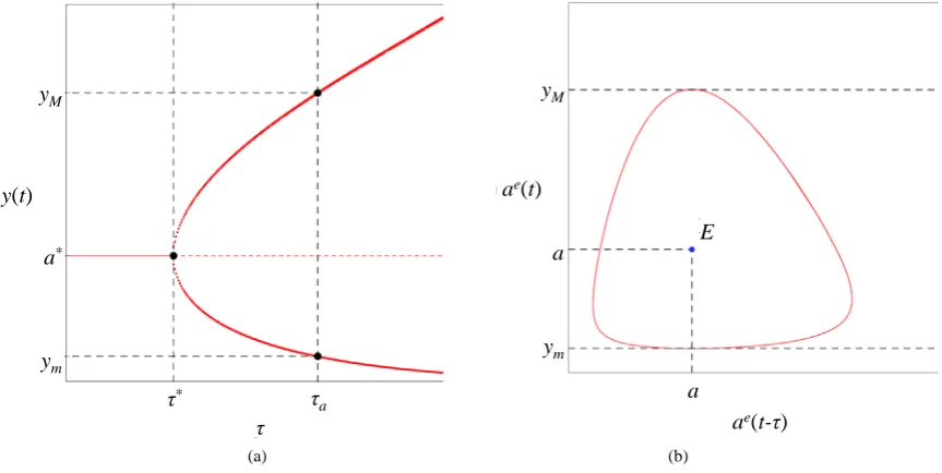
curve defined by Equation (8) with n=1 where the real part of another eigenvalue changes its sign to positive from negative. Repeating the same arguments, we see that at each intersection one more eigenvalue changes its real part from negative to positive, so stability cannot be regained and therefore no stability switch occurs for any n≥1. Hence stability is changed only when τ crosses the partition curve.Theorem 1 is numerically confirmed. Given a=2, a bifurcation diagram with respect to τ is depicted in Figure1(a). It is seen that the steady state loses stability at τ τ= ∗ and bifurcates to a cyclic oscillation for τ τ> ∗
150
are denoted by yM and ym. Figure 1(b) illustrates a limit cycle having the same extremum in the phase plane.
We can discuss another delay adjustment process that is a hybrid of Equations (4) and (5),
( )
( )
(
( ) (
1) (
)
)
e e e e
a t =ka t a− ωa t + −ω a t−τ (9)
where ω is a positive constant less than unity. It can be seen that Equation (9) is reduced to Equation (4) when ω goes to unity and to Equation (5) when ω goes to zero. The steady state of Equation (9) is equal to the maximum price and thus the same as the one of Equation (4) as well as Equation (5). The linearized equtaion becomes
( )
( )
(
1) (
)
0z t +αωz t +α −ω z t−τ =
and its characteristic equation is
(
1)
e λτ 0 λ αω α+ + −ω − =.
Using the similar arguments, we can obtain the results including that the delay becomes harmless if the instan-teneous term ae
( )
t is dominant in Equation (9):Theorem 2: 1) If ω ≥1 2, then the steady state of the hybrid logistic adjustment process (9) is locally asymptotically stable for all delay τ≥0;2) if ω <1 2, then the steady state is locally asymptotically stable if τ τ< ∗
, loses stability for τ τ= ∗ and bifurcates to a limit cycle via a Hopf bifurcation if τ τ> ∗ where
1
1 1 2
sin 1 1 2
ak
ω τ
ω ω
∗= − −
−
− .
3. Delay Discrete Dynamics
Our concern in this section is on how the different choice of the time scale affects dynamics examined in the previous section. Toward this end, we discretize the delay differential Equation (4) by replacing ae
( )
t with(
1)
( )
e e
a t+ −a t to obtain
(
1)
( )
( )
(
(
)
)
e e e e
a t+ =a t +ka t a a− t−τ (10)
and then reconsider local and global dynamics in discrete time. The positive steady state of Equation (5) remains as a steady state of this difference equation. We mention that this discrete-time equation has a τ -step delay
[image:5.595.98.530.486.703.2]
(a) (b)
Figure 1. Cyclic oscillations for τ τ> ∗. (a) Bifurcation diagram; (b) Limit cycle with τ τ= a. y(t)
a*
τ* τa
τ ym
yM
ae(t)
ym
a E
ae(t-τ) yM
151 when τ ≥12
. The remaining of this section starts with the case of τ =0 and then, proceed the cases of τ≥1 in detail to concentrate on delay effects in the discrete-time framework.
If τ=0, then Equation (10) becomes a nonlinear first-order difference equation
(
1)
( )
( )
(
( )
)
x t+ =x t +kx t a−x t (11)
where we introduce the new variable x=ae. Changing the variable again by
1 x z
ak k
= +
reveals that Equation (11) can be reduced to the familiar form,
(
1) (
1) ( )
(
1( )
)
z t+ = +ak z t −z t .
It is now well known that the logistic equation can generate wide variety of dynamics ranging from a periodic cycle to chaos according to the specification of the coefficient 1+ak if the steady state is locally unstable.
If τ=1, then Equation (10) has one-step delay and then becomes a nonlinear second-order difference equa-tion
(
1) ( )
( )
(
(
1)
)
x t+ =x t +kx t a−x t− (12)
which can be converted to an equivalent 2D system of first-order difference equations,
(
)
( )
(
) (
) ( )
( ) ( )
1 ,
1 1 .
y t x t
x t ak x t kx t y t
+ =
+ = + − (13)
The linearized system around the steady state x= =y a is
(
)
(
)
( )
( )
1 1
1 1 0
x t ak x t
y t y t
δ δ
δ δ
+ −
=
+
where the subscript δ implies that the variable with this subscript is the difference between its value and the steady state. The characteristic equation is transformed into a quadratic equation,
2
0 ak
λ − +λ = . (14) The following three conditions imply that the quadratic polynomial 2
1 2
a a
λ + λ+ has roots inside the unit cycle,
1 2
1 2
2
1 0,
1 0,
1 0
a a
a a
a + + > − + > − >
(15)
where
1 1 and 2
a = − a =ak.
The first and second conditions of Equation (15) are always satisfied and so is the third condition if and only if 1.
ak<
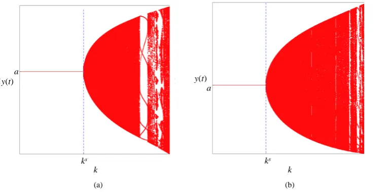
Taking a=2 and selecting k as the bifurcation parameter, we illustrate the bifurcation diagram in Figure 2(a) in which stability of the steady state is changed to instability at ks =1 a
(
=0.5)
and cyclic behavior emerges for sk>k When k arrives at k0.635, the non-negativity condition is violated resulting in the birth of economically uninteresting behavior.
We further extend our analysis to a two-step delay (i.e., τ =2) where the marginal revenue includes the de-layed information obtained at period t−2. The dynamic Equation (10) is now a third-order difference equation,
(
1)
( )
( )
(
(
2)
)
x t+ =x t +kx t a−x t− . (16)
2A sailent feature of a discrete-time equation is that the equation involves at least one difference or time-delay of the dependent variable. So
152
This can be written as a 3D system of first-order difference equations
(
)
( )
(
)
(
) (
) ( )
( ) ( )
1
1
1 1
y t x t
z t yt
x t ak x t kx t z t
+ = + =
+ = + −
(17)
where the steady state is
(
x y z, ,)
with x= = =y z a. Linear approximation of Equations (17) yields the li-nearized system having the form(
)
(
)
(
)
( )
( )
( )
1 1 0
1 1 0 0
1 0 1 0
x t ak x t
y t y t
z t z t
δ δ
δ δ
δ δ
+ −
+ =
+
(18)
and the corresponding characteristic equation is cubic,
3 2
0 ak
λ −λ + = . (19) The steady state is locally asymptotically stable if all eigenvalues of Equation (19) are less than unity in absolute value. Farebrother [7] has proved that the most simplified form of the sufficient and necessary conditions for the cubic equation 3 2
1 2 3
a a a
λ + λ + λ+ to have roots only inside the unit cycle are
1 2 3
1 2 3
2
2 1 3 3
2
1 0,
1 0,
1 0,
3
a a a
a a a
a a a a
a
+ + + >
− + − >
− + − >
<
(20)
where
1 1, 2 0 and 3
a = − a = a =ak
It can be verified that the first and fourth conditions are always satisfied while the second and third condition holds if
5 1
0.618 2
ak< − .
The bifurcation diagram with a=1 is illustrated in Figure2(b), where ks 0.618. It can be seen that Hopf bifurcation emerges for k>ks.
If τ =3, then the characteristic equation is λ4−λ3+ =α 0 with α=ak. For the quartic equation
4 3 2
1 2 3 4 0
a a a a
λ + λ + λ + λ+ =
[image:7.595.121.504.514.704.2]
(a) (b)
Figure 2. Bifurcation diagrams with different steps, (a) τ = 1 and a= 2; (b) τ = 2 and a= 1.
a y(t)
ks
k
y(t)
a
ks
the sufficient and necessary condition that all roots are inside the unit circle are (see Farebrother, [7]) as follows:
(
)
(
( )
)
(
) (
)(
)
4
4 2
1 2 3 4
1 2 3 4
2 2
4 4 2 4 1 3 3 1 4
1 0
3 3
1 0
1 0
1 1 1 0
a
a a
a a a a
a a a a
a a a a a a a a a
− > + >
+ + + + >
− + − + >
− − − − + − − >
To our case, a1= −1,a2 =a3 =0 and a4=α. The first four conditions are clearly satisfied if α<1 and the
last condition can be reduced to the following:
( )
3 22 1 0
f α =α −α − α+ > .
Clearly
( )
1 1,( )
0 1,( )
1 1,( )
and( )
f − = f = f = − f −∞ = −∞ f ∞ = ∞.
Since f′
( )
α =3α2−2α−2 having two roots1 2
1 7 1 7
0.548 and 1.215
3 3
α = − − α = + ,
( )
f α increases in intervals
(
−∞,α1)
and(
α2,∞)
, and decreases in(
α α1, 2)
. Notice that f( )
α1 >0 and( )
2 0f α < , so f
( )
α has three real roots: one is negative, two positive in intervals( )
0,1 and(
α2,∞)
. Since 1α< and the smallest positive root is approximately 0.4453, the stability condition is k<0.445. It is numer-ically confirmed that the steady state is violated via Neimark-Sacker bifurcation for k>0.445. Although the critical values s
k seem to decrease as the value of τ increases,
1 if 1, 0.618 if 2 and 0.445 if 3
s s s
k = τ= k τ= k τ = ,
this fact has not been analytically confirmed yet.
Applying the same argument to the case of the general case, we have the adjustment process described by a
(
τ+1 th)
-order difference equation,(
1)
( )
( )
(
(
)
)
x t+ =x t +kx t a−x t−τ
and a
(
τ +1 th)
-order characteristic equation,1
0 ak
τ τ
λ + −λ + =
For a larger value of τ ≥4, we do not have the simplifed stability condition but the Samuelson or the Cohn- Schur conditions for the n-th order equation can be applied to determine the critical value of k for the birth of Neimark-Sacker bifurcation4. We summarize the main result on the delay difference adjustment process:
Theorem 3: Given the maximum price, the discrete-time adjustment process (10) has the critical value of the adjustment coefficient s
k and the steady state is locally asymptotically stable if s
k<k , loses stability for s
k=k and bifurcates to a limit cycle via Neimark-Sacker bifurcation if s k>k .
4. Concluding Remarks
In this study, we analyzed the delay dynamics of a nonlinear monopoly. Two conventional assumptions in the traditional monopoly model are modified: the information obtained from the market is assumed to be limited and delayed. As a natural consequence, the monopoly is unable to jump, with one shot, to the optimal point but
3With Mathematica, it can be found that the critical value has the following form,
(
)
(
)
(
) (
)
1 32 3
1 3 2 3
7
1 3 1 3 3
7 1 3
1 2 0.445
3 3 2 1 3 3 6
s
i i
i k
i
+ − +
+
= − −
× − + .
4The forms of both conditions are found in Gandolfo [8]. In either from, the stability condition becomes complicated as the order of the
154
revises its decision by taking transaction data experiences obtained from the market into account. In either the continuous-time framework or the discrite-time framwork, the steady state is locally asymptotically stable for the smaller values of delay and bifurcates to a limit cycle via a Hopf bifurcation in the continuous-time frame-work and via a Neimark-Sacker bifurcation in the discrete-time frameframe-work for the larger values. Delay mono-poly generates very different dynamics than those of the text-book monomono-poly.
Acknowledgements
The authors highly appreciate the financial supports from the MEXT-Supported Program for the Strategic Re-search Foundation at Private Universities 2013-2017, the Japan Society for the Promotion of Science (Grant-in-Aid for Scientifc Research (C) 24530201 and 25380238) and Chuo University (Grant for Special Re-search). The usual disclaimers apply.
References
[1] Puu, T. (1995) The Chaotic Monopolist. Chaos, Solitions and Fractals, 5, 35-44.
http://dx.doi.org/10.1016/0960-0779(94)00206-6
[2] Naimzada, A.K. and Ricchiuti, G. (2008) Complex Dynamics in a Monopoly with a Rule of Thumb. Applied Mathe-matics and Computation, 203, 921-925. http://dx.doi.org/10.1016/j.amc.2008.04.020
[3] Asker, S.S. (2013) On Complex Dynamics of Monopoly Market. Economic Modeling, 31, 586-589.
http://dx.doi.org/10.1016/j.econmod.2012.12.025
[4] Matsumoto, A. and Szidarovszky, F. (2013) Complex Dynamics of Monopolies with Gradient Adjustment. IERCU DP # 209, Institute of Economic Research, Chuo University.
[5] Hayes, N.D. (1950) Roots of the Transcendental Equations Associated with Certain Difference-Differential Equation.
Journal of London Mathematical Society, 25, 226-232. http://dx.doi.org/10.1112/jlms/s1-25.3.226
[6] Matsumoto, A. and Szidarovszky, F. (2013) An Elementary Study of a Class of Dynamic System with Single Time Delay. CUBO A Mathematical Journal, 15, 1-7.
[7] Farebrother, R.W. (1973) Simplified Samuelson Conditions for Cubic and Quartic Equations. The Manchester School of Economic and Social Studies, 41, 396-406. http://dx.doi.org/10.1111/j.1467-9957.1973.tb00090.x
[8] Gandolfo, G. (2009) Economic Dyamics. 4th Edition, Springer, Berlin.