Citation:
Hanley, B and Tucker, CB and Bissas, A (2017) Differences between motion capture and video anal-ysis systems in calculating knee angles in elite-standard race walking. Journal of Sports Sciences, 36 (11). pp. 1250-1255. ISSN 1466-447X DOI: https://doi.org/10.1080/02640414.2017.1372928 Link to Leeds Beckett Repository record:
http://eprints.leedsbeckett.ac.uk/4021/
Document Version: Article
This is an Accepted Manuscript of an article published by Taylor & Fran-cis in Journal of Sports Sciences on 29 August 2017, available online: http://www.tandfonline.com/10.1080/02640414.2017.1372928
The aim of the Leeds Beckett Repository is to provide open access to our research, as required by funder policies and permitted by publishers and copyright law.
The Leeds Beckett repository holds a wide range of publications, each of which has been checked for copyright and the relevant embargo period has been applied by the Research Services team.
We operate on a standard take-down policy. If you are the author or publisher of an output and you would like it removed from the repository, please contact us and we will investigate on a case-by-case basis.
1
Differences between motion capture and video analysis systems in
calculating knee angles in elite-standard race walking
Brian Hanley, Catherine B. Tucker and Athanassios Bissas
Carnegie School of Sport, Headingley Campus, Leeds Beckett University, United Kingdom
Correspondence details: Brian Hanley,
Fairfax Hall,
Headingley Campus, Leeds Beckett University, LS6 3QS,
United Kingdom.
Telephone: +44 113 812 3577 Fax: +44 113 283 3170
Email: [email protected]
Running title: Differences in calculating race walk knee angles
2 ABSTRACT
3 INTRODUCTION
Race walking is an Olympic event dictated by International Association of Athletics Federations (IAAF) Rule 230.2 that no visible loss of contact with the ground should occur and that “the advancing leg must be straightened (i.e., not bent at the knee) from the moment of first contact with the ground until the vertical upright position”
(IAAF, 2015, p. 253). This strictly-enforced rule affects the gait mechanics of the whole body (Hanley & Bissas, 2016; Pavei, Cazzola, La Torre, & Minetti, 2014) and the knee is therefore the most important joint to assess with regard to legal race walking technique. However, judging of the knee’s straightness in competition is to the human eye only and therefore entirely subjective; as a result, the definition of Rule 230.2 and its implementation are not without controversy (Osterhoudt, 2000). This is partly because of the complexity of the knee joint’s movements in dynamic
gait (Lafortune, Cavanagh, Sommer, & Kalenak, 1992), but also because there is no specific definition of what constitutes a ‘straightened’ knee (e.g., regarding joint angle magnitude). It is therefore important that the knee angle is measured correctly in race walking so that its movements are understood and can be used as part of judge education.
4
potential to more accurately measure this joint’s motion (e.g., during the combination of extension with internal rotation of the tibia). Although Alkjaer, Simonsen, & Dyhre-Poulsen (2001) found that using a 2D model of joint moments was appropriate for human gait analysis because of how similar the results produced were to a 3D model, 3D motion analysis using optoelectronic systems has become more prominent within race walking research (Cazzola, Pavei, & Preatoni, 2016; Donà, Preatoni, Cobelli, Rodano & Harrison 2009; Pavei & La Torre, 2016; Preatoni, Ferrario, Donà, Hamill, & Rodano, 2010). These optoelectronic systems tend to have the advantage that quick, precise and accurate 3D data analysis is possible, but the need for skin marker attachment means visual light systems (usually camcorders) are required if analysing competitive performances instead. 3D measurements of the knee angle during world-class race walking competitions have indeed been conducted using videography (e.g., Hanley, Bissas, & Drake, 2011), but most race walking studies have relied on video-based 2D analyses. It will therefore be useful to ascertain differences between 2D and 3D motion analysis systems when calculating the knee joint angle in race walking.
5
error is the overlying skin movement over bone that occurs to facilitate joint motion. Similar research on the elbow angle in cricket bowling (which, like race walking, has a specific rule about joint movement) suggested that soft tissue movement contributed to greater differences between video and a triad (cluster) marker system than between video and pairs of markers placed at relevant bony landmarks (Yeadon & King, 2015). Knee sagittal movements are not as affected by soft tissue movement as movements in other planes (Reinschmidt, van den Bogert, Nigg, Lundberg, & Murphy, 1997), but even small errors could be important in race walking because of its role in legal technique. Visual, markerless systems have the advantage of being usable in competitive situations, but tracking is subjective and is therefore highly dependent on the skill of the operator (Payton, 2008). The straightened knee part of IAAF Rule 230.2 means that accurate measurements of the knee are important and it will be useful to identify the differences that occur between methodologies when supporting and assessing race walkers in the biomechanics laboratory, and in terms of those systems that can be used in competition. The aim of this study was to compare the measurement of knee angles between 2D video and 3D optoelectronic systems in race walking.
METHODS
Participants
6
standard. The mean personal best time (h:min:s) for the seven men over 20 km was 1:24:13 (± 2:49), whereas for the five women it was 1:32:32 (± 2:14).
Data collection
Passive retroreflective markers (12.5 mm) were placed on 13 anatomical landmarks of the pelvis and right leg: the left and right anterior superior iliac spines (ASIS), left and right posterior superior iliac spines (PSIS), greater trochanter, lateral and medial femoral condyles, lateral and medial malleoli, calcaneus, heads of the first and fifth metatarsals, and the distal end of the second toe. The foot markers were attached to the athletes’ training shoes, and in some cases the greater trochanter marker was
attached onto tightly fitting shorts, rather than directly onto skin. In addition, rigid clusters comprising four non-collinear markers were attached to the thigh and shank body segments. To reduce measurement error from inconsistent placement of markers, these were positioned by a single experienced researcher.
Before the dynamic (race walking) trials, each participant carried out a standing calibration trial to create anatomical reference frames for each segment. After this trial, the markers on the medial femoral condyle and medial malleolus were removed. Each athlete then race walked along a 45 m indoor track at a speed equivalent to their season’s best time for 20 km, calculated using timing gates placed
7
A 12-camera Oqus 7 3D optoelectronic motion capture system (Qualisys, Gothenburg, Sweden) operating at 250 Hz captured 3D marker coordinate data of the leg markers. The optoelectronic system was calibrated using a 601.9 mm calibration wand and L-frame reference object to define the laboratory origin and global coordinate system. The calibration results indicated a mean residual marker position error of less than 1.5 mm on each testing occasion.
2D video data were collected simultaneously at 100 Hz using a high-speed camera (Fastec TS3, San Diego, CA). A 25 mm lens was used whose centre was 1.10 m above the track’s surface. The shutter speed was 1/500 s, the f-stop was 2.0, and there
was no gain. The camera was placed approximately 10 m from and perpendicular to the line of race walking. The resolution of the camera was 1280 x 1024 pixels. Four 3 m high reference poles were placed in the centre of the camera’s field of view in
the centre of the running track in the sagittal plane. The reference poles provided a total of 12 reference points (up to a height of 2 m) that were later used for calibration (scaling). The data analysed from the optoelectronic and videography systems were of the same strides for each athlete.
Data analysis
The coordinate data from the optoelectronic system were labelled through Qualisys Track Manager 2.14 (QTM). Data from QTM were treated in two separate ways; first, the three joint markers (greater trochanter, lateral femoral condyle and lateral malleolus) were used to calculate knee joint angle based on their coordinates (the ‘marker’ condition); and second, raw kinematic data were exported to Visual3D
8
incorporated the clusters (i.e., thigh and shank orientation) (the ‘3D model’ condition). The knee angles produced by the 3D model data were considered the criterion values. Both sets of knee angle data from the optoelectronic methodologies were filtered using a recursive second-order, low-pass Butterworth digital filter (zero phase-lag) with cut-off frequencies ranging from 6.1 to 10.4 Hz (found using residual analysis (Winter, 2005)). A four-segment rigid model of the right leg was constructed for each participant where movement in six degrees of freedom was determined for the local coordinate systems of all segments (pelvis, thigh, shank and foot). Each segment was given a local coordinate system and angular displacement at the knee joint was defined as rotations of the coordinate axes of the shank (distal) segment relative to the axes of the thigh (proximal) segment. The pelvis segment was derived from the location of the ASIS and PSIS markers, and the hip joint centre was calculated according to the procedures described by Bell, Pedersen, & Brand (1990). The frontal plane for the thigh was defined by the hip joint centre at the proximal endpoint and the lateral and medial femoral condyle markers at the distal end. The frontal plane for the shank was defined by the thigh distal endpoint (proximal end) and the two malleolus markers (distal end). The frontal plane of the foot was defined by the two malleolus markers (proximal end) and the projection on the floor of the two malleolus markers (distal end).
The video files were digitised in two ways: first, through manually digitising (SIMI Motion 9.0.3, Munich) by a single experienced operator (the ‘manual’ condition); and second, using SIMI Motion’s automatic tracking function to track the three
9
started at least 10 frames before the beginning of the stride and completed at least 10 frames after to provide padding during filtering (Smith, 1989). For the manual condition, each video was first digitised frame by frame and adjustments made as necessary using the points over frame method (Bahamonde & Stevens, 2006). The manually digitised points were not necessarily on the markers themselves but chosen based on visual inspection. On a small number of occasions during automatic tracking, marker dropout occurred (e.g., because the hand obscured the greater trochanter marker) and corrections were made manually; this process of manual corrections was also made during the reliability tests that are described below. The segment endpoints used to calculate the knee joint were the hip joint, knee joint, and ankle joint. A recursive second-order, low-pass Butterworth digital filter (zero phase-lag) was used to filter the raw knee angle data. The cut-off frequencies were calculated using residual analysis (Winter, 2005) and ranged between 7.9 and 10.6 Hz (manual) and between 8.1 and 10.3 Hz (tracking).
10
mean square (RMS) difference between the original and altered files for one complete stride was 0.14° for the hip marker, 0.29° for the knee marker and 0.30° for the ankle marker. The RMS difference between the original and altered files when all three markers were moved one pixel posteriorly was 0.17°.
The knee angle was calculated as the sagittal plane angle between the thigh and lower leg segments, and rounded to the nearest integer (except when reporting the very small reliability values found above). Knee angles were considered to be 180° in the anatomical standing position, and angles beyond this as hyperextension. The knee angle has been presented in this study at specific events of the gait cycle as defined below:
Initial contact – for the video system, this was the first visible point during stance where the athlete’s foot clearly contacts the ground (heel strike). For the
optoelectronic system, heel strike was considered to occur when the vertical acceleration of the heel marker reached its minimum magnitude during the downwards movement of the foot.
Midstance – for the video system, this was a visually chosen position where the athlete’s foot was directly below the hip, used to determine the ‘vertical upright position’ (IAAF, 2015). For the optoelectronic system, midstance was considered
to occur when the hip joint centre was positioned directly above the foot centre of mass (found using the model created using Visual3D).
Statistical analysis
11
across their five trials, and then averaged across all participants. One-way analysis of variance (ANOVA) was conducted with post-hoc Tukey tests to establish significant differences between conditions (Field, 2009). An alpha level of 5% was set for these tests. Where differences between pairs of methodologies were found, effect sizes (ES) were calculated using Cohen’s d (Cohen, 1988) and considered to be either trivial (ES ≤ 0.20), small (0.21 – 0.60), moderate (0.61 – 1.20), large (1.21 – 2.00), or very large (2.01 – 4.00) (Hopkins, Marshall, Batterham, & Hanin, 2009). Differences and 95% confidence intervals (95% CI) have been reported only when the ES was moderate or larger.
RESULTS
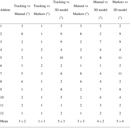
The mean race walking speed for all athletes during testing was 13.62 km·h-1 (± 0.73). The knee angle curves during a complete gait cycle for each condition are shown in Figure 1. The mean RMS differences between conditions for the stance phase for each individual athlete and for the whole group are shown in Table 1.
The mean angle at initial contact was 180° (± 2) using manual digitising, 180° (± 4) using tracking, 180° (± 4) using markers, and 183° (± 5) using the 3D model; there were no differences found between conditions. The mean angle during midstance was 184° (± 5) using manual digitising, 181° (± 6) using tracking, 181° (± 6) using markers and 187° (± 5) using the 3D model. The angle found using the 3D model was larger than that found using tracking (P = 0.048, ES = 1.04, 95% CI = 0.04 to 12.22) and markers (P = 0.034, ES = 1.13, 95% CI = 0.36 to 12.53).
12 **** Table 1 near here ****
DISCUSSION
The aim of this study was to compare the measurement of knee angles between 2D video and 3D optoelectronic systems in race walking. Overall, there was little difference between most motion analysis systems, although the gold-standard 3D model differed from the tracking and marker conditions when calculating midstance angles, and highlighted the limitation of modelling knee joint angular motion using three joint centre markers only. The 3D model also had the greatest RMS differences in comparisons with the other methodologies during stance. These differences might have occurred because the deep-lying hip joint centre was located using several markers in the 3D model rather than just the greater trochanter marker in the tracking and marker conditions, notwithstanding that the knee and ankle joints were also located slightly differently in the 3D model. It was unsurprising that the tracking function in SIMI Motion and markers in QTM produced similar knee angles given their values were based on the same three joint markers; the difference of 6° at midstance for both conditions from what was found using the 3D model showed that the clusters and extra single markers used in the 3D model were invaluable in achieving more precise, accurate angles, and should be used whenever possible if optoelectronic systems are being used.
13
14
differences between manual digitising and the 3D model ranged from 1° to 8°, and thus it should be noted that greater errors can occur with either system on some occasions. Even during automatic tracking, manual corrections were made when marker dropout occurred (mostly when the hand or arm obscured the view of the greater trochanter marker) and this process helped improve the reliability found for automatic tracking. It is therefore important for those researchers who capture data in competition to become skilled at manual digitising, through considerable prior practice and excellent anatomical knowledge.
The stance phase is the most important to analyse in race walking because technical legality is assessed between initial contact and midstance only. Race walkers typically adopt a narrow stride width (Hanley & Bissas, 2016; Pavei & La Torre, 2016) that results from hip adduction; the present study has shown that this frontal plane movement of the athletes’ lower limbs might have been what caused greater
differences between systems at midstance than at initial contact, and shows the importance of using clusters of markers where possible. Regarding other movements, transverse plane movements of the knee are restricted during stance in race walking because of its extended (or hyperextended) position, and although Graci & Salsich (2016) found transverse plane differences between a 3D model that included a greater trochanter marker and one without it, differences were small for knee sagittal plane movements, and the authors concluded that models with or without the greater trochanter could therefore be used interchangeably. Although the constraints on the knee’s movement during stance in race walking (in all planes) mean that skin
15
gait such as running where the knee flexes and extends considerably during the contact phase, and thus more caution might be warranted if analysing such activities.
IAAF Rule 230.2 does not define a straightened leg other than to state that is should not be “bent at the knee”; the results of this study showed that the mean knee angle at
initial contact was at least 180° (there was no difference between methodologies), and given that this mean value is similar to that found in world-class competition (Hanley et al., 2011), in laboratory settings using high-speed cameras (Padulo et al., 2013), and using markers (Pavei & La Torre, 2016), it seems reasonable to adopt this value as a robust guide for knee ‘straightness’ in race walking. As the race walkers in
16
manual 3D digitising condition in future studies could be beneficial in further evaluating differences between visual and optoelectronic motion analysis systems. In addition, there is no research to date on what magnitude of knee angles appear “straightened” (or not) to race walk judges, although research on race walkers in
competition (who were not disqualified) found initial contact angles ranged between 174° and 183° (20 km women), 177° and 184° (20 km men), and 175° and 186° (50 km men) (Hanley et al., 2011; Hanley et al., 2013). Future studies that assess this could be useful not only with regard to improved judging, but also in terms of calculating the size of the smallest worthwhile difference (Hopkins, Hawley, & Burke, 1999) between analysis systems.
CONCLUSIONS
17 REFERENCES
Alkjaer, T., Simonsen, E. B., & Dyhre-Poulsen, P. (2001). Comparison of inverse dynamics calculated by two- and three-dimensional modules during walking. Gait and Posture, 13, 73-77. doi: 10.1016/S0966-6362(00)00099-0
Bahamonde, R. E., & Stevens, R. R. (2006). Comparison of two methods of manual digitization on accuracy and time of completion. Proceedings of the XXIV International Symposium on Biomechanics in Sports, 24, 650-653. Retrieved from https://ojs.ub.uni-konstanz.de/cpa/article/view/207/167
Bartlett, R., Bussey, M., & Flyger, N. (2006). Movement variability cannot be determined reliably from no-marker conditions. Journal of Biomechanics, 39, 3076-3079. doi: 10.1016/j.jbiomech.2005.10.020
Bell, A. L., Pedersen, D. R., & Brand, R. A. (1990). A comparison of the accuracy of several hip center location prediction methods. Journal of Biomechanics, 23, 617-621. doi: 10.1016/0021-9290(90)90054-7
Cazzola, D., Pavei, G., & Preatoni, E. (2016). Can coordination variability identify performance factors and skill level in competitive sport? The case of race walking. Journal of Sport and Health Science, 5, 35-43. doi: 10.1016/j.jshs.2015.11.005
18
Cutti, A. G., Cappello, A., & Davalli, A. (2006). In vivo validation of a new technique that compensates for soft tissue artefact in the upper-arm: Preliminary results. Clinical Biomechanics, 21, S13-S19. doi: 10.1016/j.clinbiomech.2005.09.018
Donà, G., Preatoni, E., Cobelli, C., Rodano, R., & Harrison, A. J. (2009). Application of functional principal component analysis in race walking: an emerging methodology. Sports Biomechanics, 8, 284-301. doi: 10.1080/14763140903414425
Field, A. P. (2009). Discovering statistics using SPSS (3rd edn.). London: Sage.
Graci, V., & Salsich, G. B. (2016). The use of the greater trochanter marker in the thigh segment model: implications for hip and knee frontal and transverse plane motion. Journal of Sport and Health Science, 5, 95-100. doi: 10.1016/j.jshs.2015.01.002
Hanley, B., & Bissas, A. (2017). Analysis of lower limb work-energy patterns in world-class race walkers. Journal of Sports Sciences, 35, 960-966. doi: 10.1080/02640414.2016.1206662
19
Hanley, B., Bissas, A., & Drake, A. (2013). Kinematic characteristics of elite men’s 50 km race walking. European Journal of Sport Science, 13, 272-279. doi: 10.1080/17461391.2011.630104
Hanley, B., Bissas, A., & Drake, A. (2011). Kinematic characteristics of elite men’s and women’s 20 km race walking and their variation during the race. Sports
Biomechanics, 10, 110-124. doi: 10.1080/14763141.2011.569566
Hoga, K., Ae, M., Enomoto, Y., & Fujii, N. (2003). Mechanical energy flow in the recovery leg of elite race walkers. Sports Biomechanics, 2, 1-13. doi: 10.1080/14763140308522804
Hopkins, W. G., Hawley, J. A., & Burke, L. M. (1999). Design and analysis of research on sport performance enhancement. Medicine and Science in Sports and Exercise, 31, 472-485. doi: 10.1097/00005768-199903000-00018
Hopkins, W. G., Marshall, S. W., Batterham, A. M., & Hanin, J. (2009). Progressive statistics for studies in sports medicine and exercise science. Medicine and Science in Sports and Exercise, 41, 3-12. doi: 10.1249/MSS.0b013e31818cb278
IAAF (2015). Competition rules 2016-17. Monte Carlo: IAAF.
20
Osterhoudt, R. G. (2000). The grace and disgrace of race walking. Track Coach, (153), 4880-4883.
Padulo, J., Annino, G., D’Ottavio, S., Vernillo, G., Smith, L., Migliaccio, G. M., &
Tihanyi, J. (2013). Footstep analysis at different slopes and speeds in elite racewalking. Journal of Strength and Conditioning Research, 27, 125-129. doi: 10.1519/JSC.0b013e3182541eb3
Pavei, G., Cazzola, D., La Torre, A., & Minetti, A. E. (2014). The biomechanics of race walking: literature overview and new insights. European Journal of Sport Science, 14, 661-670. doi: 10.1080/17461391.2013.878755
Pavei, G., & La Torre, A. (2016). The effects of speed and performance level on race walking kinematics. Sports Sciences for Health, 12, 35-47. doi: 10.1007/s11332-015-0251-z
Payton, C. J. (2008). Motion analysis using video. In C. J Payton, & R. M. Bartlett (Eds.), Biomechanical evaluation of movement in sport and exercise: The British Association of Sport and Exercise Sciences guidelines (pp. 8-32). Abingdon: Routledge.
21
Reinschmidt, C., van den Bogert, A. J., Nigg, B. M., Lundberg, A., & Murphy, N. (1997). Effect of skin movement on the analysis of skeletal knee joint motion during running. Journal of Biomechanics, 7, 729-732. doi: 10.1016/S0021-9290(97)00001-8
Sinclair, J., Richards, J., Taylor, P. J., Edmundson, C. J., Brooks, D., & Hobbs, S. J. (2013). Three-dimensional kinematic comparison of treadmill and overground running. Sports Biomechanics, 3, 272-282. doi: 10.1080/14763141.2012.759614
Smith, G. (1989). Padding point extrapolation techniques for the Butterworth digital filter. Journal of Biomechanics, 22, 967-971. doi: 10.1016/0021-9290(89)90082-1
White, S. C., & Winter, D. (1985). Mechanical power analysis of the lower limb musculature in race walking. International Journal of Sport Biomechanics, 1, 15-24. doi: 10.1123/ijsb.1.1.15
Winter, D. A. (2005). Biomechanics and motor control of human movement (3rd ed.). Hoboken, NJ: John Wiley & Sons.
22
Table 1. RMS differences in knee angle for the four conditions during stance for the 12 race walkers.
Athlete
Tracking vs Manual (°)
Tracking vs Markers (°)
Tracking vs 3D model
(°)
Manual vs Markers (°)
Manual vs 3D model
(°)
Markers vs 3D model
(°)
1 3 1 3 3 2 2
2 8 1 9 8 2 9
3 2 1 9 2 7 9
4 1 2 4 2 4 4
5 2 1 10 3 8 11
6 1 2 2 1 1 2
7 5 3 8 8 4 11
8 6 1 2 6 4 2
9 1 1 8 2 7 8
10 2 1 5 2 6 4
11 2 1 1 2 3 2
12 1 1 2 1 2 2
23
[image:24.595.137.476.238.489.2]