A STUDY OF WELDING PROCESS USING THE TAGUCHI EXPERIMENTAL DESIGN TECHNIQUE

(1)

GE-International Journal of Engineering Research

Vol. 3, Issue 12, Dec 2015 IF- 4.007 ISSN: (2321-1717) © Associated Asia Research Foundation (AARF) Publication

Website: www.aarf.asiaEmail : [email protected] , [email protected]

A STUDY OF WELDING PROCESS USING THE TAGUCHI

EXPERIMENTAL DESIGN TECHNIQUE

Pavel Blecharz1, Ranjit K. Roy2

1

Faculty of Economics, VSB-Technical University of Ostrava, Sokolska 33, 70121 Ostrava, Czech Republic.

2

Nutek, Inc., 3829 Quarton Road, Bloomfield Hills, MI 48302, USA.

ABSTRACT

This report presents a study to improve a welding process used in production of an

automotive component. For this experimental study, the method known as the Design of

Experiments using Taguchi approach was used. The results of the experiments were

evaluated with two quality characteristics with opposing direction of desirabilities. By

performing two experiments and the subsequent separation of factors into 4 groups, it was

possible to achieve an optimum design in which both the characteristics satisfied the

customer requirements.

Keywords

Design of experiments, process improvement, quality, Taguchi, welding. 1 Introduction

Proper quality management for manufacturing organization has been a rewarding activities for last several decades. Companies that devoted attention to improving quality, are known to have earned higher return on investment. In light of today's competitive market, improvement in quality of products and services is crucial for business survival.

(2)

production process, focus for improvement is shifted toward building quality into the product and process upfront in the design and development phase. For last three decades, the statistical techniques known as Design of Experiments (DOE) using the Taguchi approach has been successfully utilized by manufacturing industries worldwide for design improvement as well as for production problem solving.

Design of Experiments using Taguchi approach is standardized form of experimental design (classical DOE). So called classical DOE was introduced by R. A. Fisher in England in the 1920's. Japanese expert Dr. Genichi Taguchi started to simplify and standardize this experimental technique after World War II for Japanese industrial productions. Over time, the method began to be used in Japanese industry and in recent days it is used mainly in automotive industry in the US and around the world.

This paper describes a way of problem solving in production by use of DOE/Taguchi technique. Solution of the problem is shown in a simplified case study which involves overall quality of welding process. Hereafter, term DOE will be used in text to represent DOE using the Taguchi approach.

2 Method Overview

DOE technique is relatively complex compared to other quality approaches. However, its use may bring dramatic quality improvement and cost reduction. Below are brief descriptions of some of the important points of DOE which are utilized in this study. For more information as for DOE technique it is possible to use further reading, e.g. [1], 1995, [2], [3] and many more.

2.1 Fundamental Terms

Quality characteristic (QC or Y) defines and measures results in terms of product and process features or evaluation criteria such as hardness, weight, strength, fault frequency, failure life, etc. From mathematical point of view, it is the dependent variable that captures influence, this is, its value depends of factors and their value setting. QC can be composed of single or multiple criteria of evaluations.

(3)

Whereas the discrete factors are like type of material, operator male/female, option yes or no, etc. Further, factors that can be adjusted for improvement are called controllable factors and those that cannot be adjusted are called uncontrollable or noise factors.

Experimenting with factors is a direct way to observe effects of factors. To study effects of factors, each must be tested least in two levels. Since, most products and processes in the industrial settings involve many factors, number of experiments required to include effects of all factor levels generally become prohibitively large. Fortunately, Taguchi approach allows use of a set of tables, called orthogonal arrays, that often reduces the number of experiments in a study to a practicable few. When analyzed, the results of the experiments based on the Taguchi orthogonal arrays leads to statistically valid conclusions.

Levels are values of the factors that are used to describe and carry out the experiments. Levels of factors are designated as A1 (factor A at level 1), A2 (factor at level 2).

2.2 Experimental Procedure

Experimental procedure consists of 5 phases: I. Experiment Planning

II. Experiment Design

III. Conducting Trial Conditions IV. Analysis of Results

V. Confirmation of Predicted Performance

I. Planning of experiments is the most important first step. The project team must discuss, deliberate and determine quality characteristic, factors and number of levels, values of setting, etc. before designing the experiment. Use of brainstorming is strongly recommended here.

(4)

[image:4.595.71.345.487.627.2]

Table 1 Orthogonal Array L4 (adapted from the source [4])

column

experiment #

1 2 3

1

2

3

4

1

2

2 1

2

1

2 1

2

1

Description of array notations:

 L represents the array (originates from Latin squares).

 Digit (e.g. 4) as the subscript of L indicates number of rows (experiments) in the array  Columns 1, 2 & 3 represent the location of factors assigned to the column.

 Digits 1 and 2 in the body of the table of numbers (array) represent levels of the factor assigned to the column.

 Numbers 1, 2, 3 & 4 represent the trial conditions as described by reading across the rows in terms of level descriptions.

In a study involving three 2-level factors, A, B & C, an experiment can be design by assigning factor A to column 1, factor B to column 2 and factor C to column 3 (see Table 2).

Table 2 L4 Experiment Design Column

Trial Conditions

1

A 2

B 3

C

Results

(or Average)

1

2

3

4

1

2

2 1

2

1

2 1

2

1

Y1 Y2 Y3 Y4

(5)

Since L4 array has three columns, only three factors can be studied using the array. In case, there are only two factors, in other words, factor C is absent, the same array can be used by keeping the third (or any other) column unassigned. The unused column, in this case, is transformed by replacing all level notations to 0.

Of course not all studies will be limited to only three factors or all factors at 2-level. This is why Taguchi has created a large number of orthogonal arrays that allows experiment designs to study larger number of factors and factors at levels more than two. While there are special set of arrays suitable for studies with 3-level and 4-level factors, often an array can be modified to accommodate 3-level and 4-level factors along with many 2-levell factors. Most frequently used arrays for 2-level factors are:

L-4 (23) ………….. 2-3 factors L-8 (27) …………...4-7 factors

L-12 (211) …………8-11 factors (special orthogonal array) L-16 (215) …………8-15 factors

L-32 (231) …………16-31 factors

All but L-12 orthogonal arrays shown above allows study of interaction between two level factors which requires reserving appropriate columns for the same. To facilitate experiment designed with knowledge of confounding effects of interaction, Taguchi offers triangular table to help with experiment design.

III. While conducting trial conditions, it is desirable to carry out the tests by selecting the trial conditions in random order rather than in sequence, upward or downward. It is also, highly desirable, to run multiple samples in the same trial condition for the sake of capturing variability in results.

IV. Analysis of results

(6)

a. Optimum condition (using average and main effects). Calculation of factor average effect for L4 array:

2 / )

( 1 2

1 Y Y

A   (factor A is at level 1 during trials 1 and 2, see table 2) 2

/ ) ( ₃ ₄

2 Y Y

A   (factor A is at level 2 during trials 3 and 4, see table 2)

Similarly, average effects of other factors are calculated. The average effects for the two levels of a factor are then compared, and based on the three common types of quality characteristic, as defined below, the optimum level for the factor is then selected.

 Type "S" (smaller is better, target value is 0),

 Type "B" (alternatively type L) (bigger/larger is better, target value is +),  Type "N" (nominal is best, target value is usually midpoint of tolerance zone).

Main effect is difference between level 2 and level 1 for average effect:

Main effect of factor A = A₂ A₁

Main effect describes relative factor influence and is measured by subtracting average effects at level 1 from that at level 2. The absolute values of the differences are compared to order the significance factor influences in relative terms. However, for specific influence of a factor in terms of percentage, calculation for following the ANOVA statistics must be performed.

b. Factor Influences in % (ANOVA)

ANOVA (Analysis Of Variance) is a standard statistical technique used to determine relative influence of the factors. ANOVA allows calculation of variances in experimental results due to factors setting (known sources of variability) and due to other influences (unknown sources of variability, i.e. experimental error).

(7)

Table 3 Table ANOVA (adapted from the source [5])

Factors f S V F S´ P (%)

A B C error

1 1 1 0

2.25 12.25

0.25

2.25 12.25

0.25

- - -

15.25 83.05 1.7

total 3 100%

f =degrees of freedom, S = sum of squares, V = mean square (variance), F = variance ratio, S´ = pure sum of squares, P = percent contribution

As we can see in column "P" (right side) shows the percent influence of the factors which indicates that factor B (83.05%) has the most influence on the variability of results. This factor is considered to have a very strong effect to quality and it needs to be kept on the right value with tight tolerances. Factor A has some influence and its level and tolerances must be set by standard practices. Factor C has the least amount of influence (less than 5 %). Such factors are usually considered insignificant allowing its level being set based on reduced costs.

c. Estimated performance (quality characteristic value) at the optimum condition

In general, the optimum determined (Step a) is different from any of the trial condition. Thus, the performance at optimum condition is estimated as shown below, which for quality characteristic type B:

) ( ) (

)

(A1 T B2 T C1 T

T

YOPT       

(where 𝑇 is sum of all experimental results divided by number of experiments)

When calculating for type S characteristic, we subtract value of average effect of factors from 𝑇 in brackets and then subtract brackets results from 𝑇 .

V. Confirmation of Predicted Performance

Following the analysis, the analytically predicted performance is verified by running tests at the optimum condition.

(8)

2.3 Experimental Results

After the trial conditions are carried out by running one or more samples, the test results are shown next to the array (see table 4). For analysis purposes, results of multiple samples are first reduced to single column of average of results or other single statistics for each trial condition.

Table 4 Experiment Results

column number of trial

1 A

2 B

3 C

results Y 1

2 3 4

1 1 2 2

1 2 1 2

1 2 2 1

12 (Y1)

9 (Y2)

14 (Y3)

10 (Y4)

For many industrial products and processes, results may be comprised of multiple criteria of evaluation each of which have different quality characteristic. Analysis of results, in such cases, may become complex. Peace [6] recommends elimination of several quality characteristics and use just one characteristic, which describe energy transfer in system. As an alternate approach, authors suggest – dividing factors into groups of factors with dominant influence to a quality characteristic.

This approach of grouping factors for study will be utilized in this study requiring increase in weld strength (quality characteristic type B) while keeping deformation thread to a minimum (quality characteristic type S).

The factor involved in the study were divided into 4 groups: a) Factors influencing just weld strength,

b) Factors influencing just deformation thread,

c) Factors influencing both, weld strength and deformation thread, d) Factors no influence on either characteristic.

(9)

purposes. The calculation based on MSD for characteristic type B (used in case study) is shown here:

MSD= [(1/Y12 + 1/Y22 +…+ 1/Y n2)] /n (1)

where Y is measured value and n = number of units in sample.

SN = -10log (MSD) [dB]1 (2)

A case study involving welding process from Czech automotive industry is presented in this report. For experiment design and analysis of results, Qualitek-4 software [7] was used in this study.

3 Case Study - Process of Electrical Welding

This experimental study was undertaken to address the customer complaints about parts not meeting the required weld strength. The aim of the experiment was to achieve the specified

weld strength while keeping the thread deformation to a minimum. Torque denoted as Ytw, was used as a measure of weld strength, quality characteristic of type B (Bigger is Better) with LSL (lower specification limit) = 40Nm. For thread deformation, quality characteristic of type S, “number of the deformed parts in 100pcs (YD)" was used as its measure. Brainstorming by the project team helped identify a number of factors with potential effects on the two quality characteristics. Factors like type of electrode, the electrode diameter, etc. were excluded from this study. Five among long list of identified factors were selected for this study (See Table 5).

Table 5 Factors And Their Levels For Electric Welding Process

Factor Level 1 Level 2

A: Flowering time (i.e. welding current growth period) 3 periods 5 periods

B: Initial current 33% 38%

C: Passage time (i.e. transit time welding current) 2 periods 4 periods

D: Welding current 46% 59%

E: Contact force (i.e. growth period of pressing force) 11 periods 14 periods

1

(10)

The experiment was designed using an L8 array and all trial conditions were run with 3 samples in each (see table 6). For analyses, the results (Table 6, R1 to R3) are first transformed to S/N ratio which are then used to determine the optimum condition and estimate the performance in decibels. Sample transformation of results (first row) is shown here:

[image:10.595.71.513.243.385.2]

MSD= [(1/49.22 + 1/49.22 + 1/49.62)] /3 = 0.000410901 SN = -10log(MSD) = 33.862dB

Table 6 Design And Results Of L8 Experiments (torque of welding) column experiment # 1 A 2 B 3 - 4 C 5 - 6 E 7 D

R1 R2 R3 SN

1 2 3 4 5 6 7 8 1 1 1 1 2 2 2 2 1 1 2 2 1 1 2 2 0 0 0 0 0 0 0 0 1 2 1 2 1 2 1 2 0 0 0 0 0 0 0 0 1 2 2 1 1 2 2 1 1 2 2 1 2 1 1 2 49.2 51.6 56.3 57.2 47.1 44.0 50.1 56.4 49.2 52.5 56.4 57.7 46.6 42.3 51.3 55.4 49.6 52.0 57,0 59,1 47.2 42.5 51.4 56.7 33.862 34.325 35.051 35.266 33.435 32.651 34.138 34.988

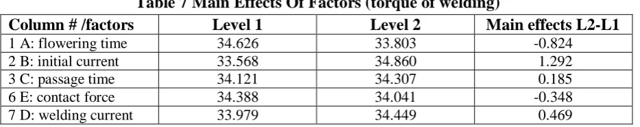
[image:10.595.66.533.469.562.2]

Calculated values of factor average effects are shown in Table 7 (further – data from software Qualitek-4 output are used).

Table 7 Main Effects Of Factors (torque of welding)

Column # /factors Level 1 Level 2 Main effects L2-L1

1 A: flowering time 34.626 33.803 -0.824

2 B: initial current 33.568 34.860 1.292

3 C: passage time 34.121 34.307 0.185

6 E: contact force 34.388 34.041 -0.348

7 D: welding current 33.979 34.449 0.469

(11)

[image:11.595.68.523.57.176.2]

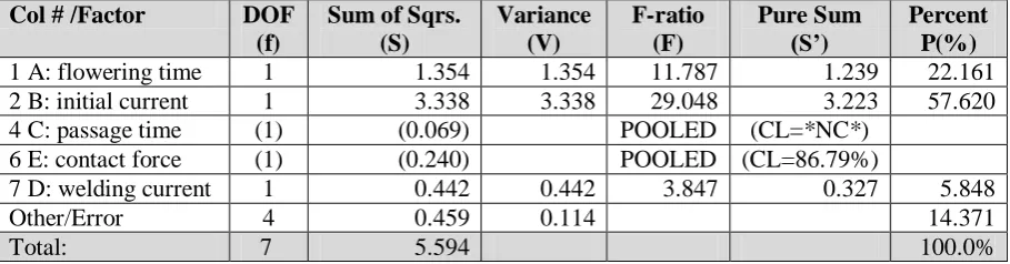
Table 8 ANOVA Table After Pooling

Col # /Factor DOF

(f)

Sum of Sqrs. (S)

Variance (V)

F-ratio (F)

Pure Sum

(S’) Percent P(%)

1 A: flowering time 1 1.354 1.354 11.787 1.239 22.161

2 B: initial current 1 3.338 3.338 29.048 3.223 57.620

4 C: passage time (1) (0.069) POOLED (CL=*NC*)

6 E: contact force (1) (0.240) POOLED (CL=86.79%)

7 D: welding current 1 0.442 0.442 3.847 0.327 5.848

Other/Error 4 0.459 0.114 14.371

Total: 7 5.594 100.0%

[image:11.595.71.509.344.448.2]

Based on three significant factors, the optimum condition is determined to be: A1 B2 D2 (see table 9). Since the performance at optimum is estimated in decibels, for practical reason, it is transformed back to the original units of measurement as shown in table 10 which is expected to be, Ytw = 59.607 Nm.

Table 9 Optimal Combination, Expected Results (torque of welding)

Column # / Factor Level Description Level Contribution

1 A: flowering time 3 periods 1 0.411

2 B: initial current 38% 2 0.646

7 D: welding current 59% 2 0.235

Total Contribution From All Factors 1.292

Current Grand average of performance 34.214

Expected Result At Optimum Condition 35.506

Table 10 Transformation To Original Unit (torque)

Formula value

S/N = -10log (MSD) 35.506

or MSD = 10^[-(S/N)/10] 0.000281

where MSD=[(1/y1)^2 + (1/y2)^2 +…+(1/yn)^2]/n

or Yexp = SQR (1/MSD) 59.607 QC units

(based on S/N=35.506 at optimum)

(12)

performance evaluated in terms of number of deformed part in 100pcs, i.e. YD (quality characteristic is the type of S), as shown in table 11.

Table 11 Design And Result of L8 Experiment (deformed parts)

column experiment # 1 A 2 B 3 - 4 C 5 - 6 E 7 D Number of deformed parts, YD

1 2 3 4 5 6 7 8 1 1 1 1 2 2 2 2 1 1 2 2 1 1 2 2 0 0 0 0 0 0 0 0 1 2 1 2 1 2 1 2 0 0 0 0 0 0 0 0 1 2 2 1 1 2 2 1 1 2 2 1 2 1 1 2 0 28 6 15 8 19 0 35

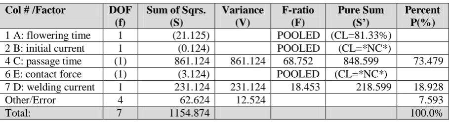
[image:12.595.67.522.388.513.2]

The ANOVA calculated based on the thread deformation results (Table 12) shows that only factors C and D have influence on this characteristic and allows determination of the optimum condition (Table 13) and the expected performance.

Table 12 ANOVA Table After Pooling (deformation)

Col # /Factor DOF

(f)

Sum of Sqrs. (S) Variance (V) F-ratio (F) Pure Sum (S’) Percent P(%)

1 A: flowering time 1 (21.125) POOLED (CL=81.33%)

2 B: initial current 1 (0.124) POOLED (CL=*NC*)

4 C: passage time (1) 861.124 861.124 68.752 848.599 73.479

6 E: contact force (1) (3.124) POOLED (CL=*NC*)

7 D: welding current 1 231.124 231.124 18.453 218.599 18.928

Other/Error 4 62.624 12.524 7.593

Total: 7 1154.874 100.0%

Table 13 Optimal Combination, Expected Results (deformation)

4 C: passage time 2 periods 1 -10.375

7 D: welding current 46% 1 -5.375

Total Contribution From All Factors -15.750

Expected Result At Optimum Condition -1.875

(13)

[image:13.595.66.531.128.272.2]

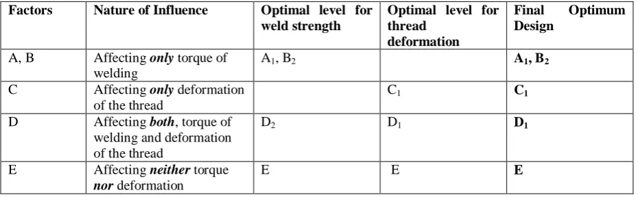
From analyses of results for both weld streangth and thread deformation, the factor influences can be established by the respective catagories defined earlier (Table 14).

Table 14. The Final Factor Adjustment From The Two Experiments

Factors Nature of Influence Optimal level for

weld strength

Optimal level for thread

deformation

Final Optimum

Design

A, B Affecting only torque of

welding

A1, B2 A1, B2

C Affecting only deformation

of the thread

C1 C1

D Affecting both, torque of

welding and deformation of the thread

D2 D1 D1

E Affecting neither torque

nor deformation

E E E

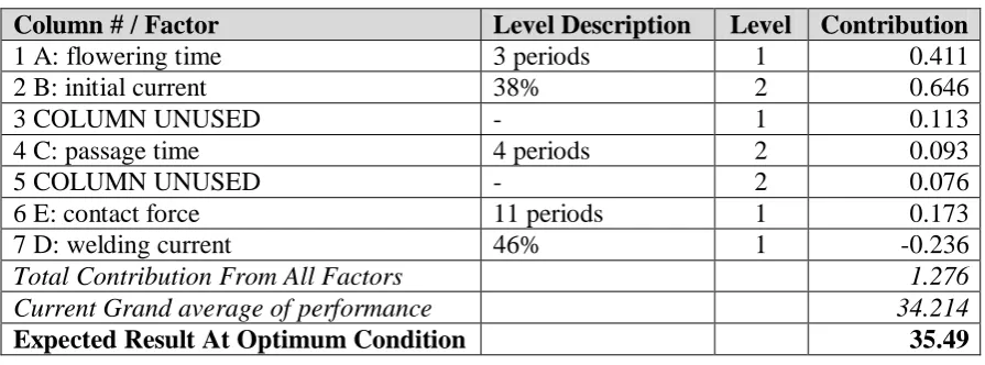
Clearly, factors A and B only affect weld strength and factor C alone has effects on thread deformation. So levels of these factors can be set to the determined levels (A1, B2 & C1) without any adjustment. At the same time, factor D affects on both characteristics, with 6% influence on weld strength (see Table 8) and 18.9% influence on thread deformation (see Table 12). For this factor, the desired level for lower thread deformation is selected for the final design while accepting a slight lowering of torque strength. Factor E, on the other hand, has no effect any of the characteristics and thus can be set either level that can potentially offer cost savings (selected E1). The final optimum design with minimum thread deformation and potential saving becomes:

A1 B2 C1D1E1

(14)

Table 15 Calculation The Torque For Adjusted Optimum

1 A: flowering time 3 periods 1 0.411

2 B: initial current 38% 2 0.646

3 COLUMN UNUSED - 1 0.113

4 C: passage time 4 periods 2 0.093

5 COLUMN UNUSED - 2 0.076

6 E: contact force 11 periods 1 0.173

7 D: welding current 46% 1 -0.236

Total Contribution From All Factors 1.276

[image:14.595.66.514.53.219.2]

References

1. W.Y. Fowlkes and C.M. Creveling, Engineering Methods for Robust Product Design
(Reading: Addison-Wesley Publishing Company, 1995).
2. R.K. Roy, Design of Experiments Using the Taguchi Approach (New York: John Wiley&Sons, 2001).
3. G. Taguchi, System of Experimental Design. Volume One (Dearborn: American Supplier Institute, 1987b).
4. G. Taguchi, Orthogonal Arrays and Linear Graphs (Allen Park: American Supplier Institute, 1987a).
5. R.K. Roy, A Primer on the Taguchi Method (Dearborn: SME, 1990).
6. G.S. Peace, Taguchi Methods. A Hands-On Approach (Reading: Addison-Wesley Publishing Company, 1993).