CONDUCTING ELASTIC HALF-SPACE IN
THERMOELASTICITY III
S. K. ROYCHOUDHURI AND NUPUR BANDYOPADHYAY
Received 21 April 2005
The propagation of magneto-thermoelastic disturbances in an elastic half-space caused by the application of a thermal shock on the stress-free bounding surface in contact with vacuum is investigated. The theory of thermoelasticity III proposed by Green and Naghdi is used to study the interaction between elastic, thermal, and magnetic fields. Small-time approximations of solutions for displacement, temperature, stress, perturbed magnetic fields both in the vacuum and in the half-space are derived. The solutions for displace-ment, temperature, stress, perturbed magnetic field in the solid consist of a dilatational wave front with attenuation depending on magneto-thermoelastic coupling and also con-sists of a part diffusive in nature due to the damping term present in the heat transport equation, while the perturbed field in vacuum represents a wave front without attenua-tion traveling with Alfv’en acoustic wave speed. Displacement and temperatures are con-tinuous at the elastic wave front, while both the stress and the perturbed magnetic field in the half-space suffer finite jumps at this location. Numerical results for a copper-like material are presented.
1. Introduction
Nowacki [11], Kaliski and Nowacki [7] considered magneto-thermoelastic waves in a perfectly electrically conducting elastic half-space in contact with a vacuum due to ap-plication of a thermal disturbance on the plane boundary. Both the half-space and the vacuum are supposed to be permeated by an applied primary uniform magnetic field. The study was made neglecting the influence of coupling between the thermal and elastic fields. Later, Massalas and Dalamangas [9,10] studied the same problem taking into ac-count the coupling of strain and temperature fields. Further, the investigation carried out in [9] was extended to TRDTE developed by Green and Lindsay [4], by Roychoudhuri and Chatterjee [3,16]. Moreover, the problem studied in [9] was also extended to ETE developed by Lord and Shulman [8], by Roychoudhuri and Chatterjee [15], and by Roy-choudhuri and Banerjee [14]. Further, Roychoudhuri and Debnath [17], Roychoudhuri [12,13] studied magneto-thermoelastic waves in a rotating solid in the context of ETE.
Copyright©2005 Hindawi Publishing Corporation
Transient magneto-thermoelastic waves in a rotating half-space were also studied in the context of ETE by Chand et al. [2].
Recently, Green and Naghdi [5,6] developed a theory where the characteristics of ma-terial response for thermal phenomena are based on three types of constitutive response functions, labeled as types I, II, and III. The nature of these three types of constitutive equations is such that when the respective theories are linearized, type I is the same as the classical heat conduction equation (based on Fourier’s law), whereas the linearized version of type II theory accommodates finite thermal wave speed and involves no dissi-pation of thermal energy. Further, the type III theory involves a thermal damping term. The mixed third-order derivative term appearing in the heat transport equation destroys the wave structure. Accordingly, this equation predicts a non-wave-like heat conduction different from the usual diffusion equation predicted by the conventional parabolic heat equation. This theory admits an infinite speed of thermal propagation. This model admits coupled damped thermoelastic waves. The purpose of the present study is to consider magneto-thermoelastic waves in an elastic half-space in contact with a vacuum due to a thermal shock applied on the stress-free plane boundary in the context of the thermoe-lasticity theory III. The medium is supposed to be a perfect electrical conductor and both media are permeated by a primary uniform magnetic field parallel to the plane boundary. Short-time solutions for displacement, temperature, stress, perturbed fields in the half-space and that in the vacuum are derived. The solutions for displacement, temperature, stress, and perturbed field in the solid consist of an elastic wave front with attenuation and a diffusive part due to the damping term present in the heat transport equation. The perturbed magnetic field in vacuum represents a wave front without any attenuation trav-eling with Alfv’en acoustic wave speed. Displacement and temperature in the half-space are found to be continuous at the elastic wave front, while the stress and the perturbed magnetic field in the solid both experience finite discontinuity at the same location. The finite discontinuities are not constants but decay exponentially with distance from the boundary.
2. Formulation of the problem and basic equations
We consider a homogeneous, isotropic, thermally and electrically conducting elastic half-spaceD:x≥0 at a uniform reference temperatureθ0in contact with a vacuumD:x <0. We suppose that in both media, there is an initial uniform magnetic field of intensityH0 acting in thez-direction so thatH0 =(0, 0,H0), whereH0 is a constant. At the instant t=0+, we assume that the stress-free plane boundaryx=0 is suddenly heated to a tem-peratureT0and left in this state.
The thermal shockT=T0H(t), whereH(t) is the Heavy-side unit step function, pro-duces in the half-space a magneto-elastic wave which depends on the spatial coordinate xand timet. At the same time, an electromagnetic wave is radiated into the vacuum [7]. The simplified linearized equations of electrodynamics of slowly moving continuous media having perfect electrical conductivity are
∇ ×h=4π
c j, ∇ × E= − µe
c ∂h
∂t, ∇ · h=0, E= − µe
c
∂u ∂t ×H0
wherehandEdenote perturbations of the magnetic and electric fields, respectively, j is the electric current density vector, H0 is the initial constant magnetic field,uis the mechanical displacement vector,µeis the magnetic permeability, andcis the velocity of
light. The displacement equations of motion in magneto-thermoelasticity are
µ∇2u+ (λ+µ)∇(divu)−γ∇T+1 c
j×B=ρu,¨ (2.2)
where (j×B) is the electromagnetic body force, Bis the magnetic induction vector,λ,µ are Lame’s constants,γ=(3λ+ 2µ)αt,αtis the coefficient of linear thermal expansion,T
is the temperature increase above the reference temperatureθ0, andρis the constant mass density.
After linearization,
j×B=j×µeH0 +h∼=µej×H0=µec
4π
∇ ×h×H0 . (2.3)
Equation (2.2), then, after linearization, reduces to
µ∇2u+ (λ+µ)∇(divu)−γ∇T+µec
4π
∇ ×h×H0=ρu.¨ (2.4)
The heat transport equation in the theory of thermoelasticity (type III) presented by Green and Naghdi [5] (in absence of heat sources) is
ρCvT¨+γθ0div ¨u=K∇2T˙+K∗∇2T, K∗>0, (2.5)
whereCvis the specific heat at constant strain,K is the thermal conductivity, andK∗
is a material constant characteristic of the theory. It may be noted that the third model represented by (2.5) of Green and Naghdi [5] for heat transport in solids accommodates infinite thermal wave speed due to the presence of third-order mixed derivative term present on the right-hand side of (2.5) and it involves thermal damping. As such, the corresponding thermoelastic model admits coupled damped thermoelastic waves.
Since the disturbances depend on the spatial coordinatexand timet, we assume, for one-dimensional deformation,
u=u(x,t), 0, 0, T=T(x,t), h=h(x,t). (2.6)
ForH0 =(0, 0,H0), (2.1) reduces to
E=0,µeH0 c u, 0˙
,
∂h ∂t =
0, 0,−H0∂u˙ ∂x
,
j=
0,− c
4π ∂hz
∂x, 0
.
The second equation of (2.7), on integration, yieldshz= −H0(∂u/∂x) for a perfect
con-ductor.
Equations (2.4) and (2.5), in one-dimensional case, for a perfect conductor simplify to
λ+ 2µ+a20ρ∂2u ∂x2−γ
∂T ∂x =ρ
∂2u ∂t2,
ρCv∂
2T
∂t2 +γθ0 ∂3u ∂x∂t2 =K
∂3T ∂x2∂t+K∗
∂2T ∂x2,
(2.8)
wherea0=µeH02/4πρis the Alfv’en wave velocity of the medium. The system of Maxwell’s equations in vacuum is expressed as
∇ ×h0=1
c ∂D0
∂t , ∇ · h
0=0, ∇ · E0=0. (2.9)
whereh0andE0are the perturbed magnetic field and the electric field in vacuum. These give
∇ ×h0=1
c ∂E0
∂t , ∇ × E 0= −1
c ∂h0
∂t . (2.10)
These equations yield the following equations satisfied byE0andh0:
∇2− 1
c2 ∂2 ∂t2
E0,h0=0. (2.11)
In one-dimensional case, this reduces to
∂2 ∂x2−
1 c2
∂2 ∂t2
E0
y,h0z)=0, (2.12)
wherex= −x.
The componentsT11andT0
11of Maxwell’s stress tensors in the elastic medium and in vacuum are given by
T11= −µe
4πhzH0, T 0 11= −
1 4πh
0
zH0. (2.13)
The total stress in the half-space is composed of Hooke’s mechanical stress and Maxwell’s stress. Thus, the total stress in the half-space is
σ∗
11=σ11+T11=(λ+ 2µ)∂u
∂x−γT+T11
=(λ+ 2µ)∂u ∂x−γT−
µe
4πhzH0
=
(λ+ 2µ) + µe 4πH
2 0 ∂u
∂x−γT,
(2.14)
Boundary conditions. (i) The continuity of total stress composed of thermoelastic and electromagnetic stress across the boundaryx=x=0 yields
σ11+T11=T110 onx=x=0. (2.15)
(ii) The tangential component ofE-field is continuous across x=x=0, which leads to
Ey=E0y onx=x=0. (2.16)
(iii) The thermal boundary condition onx=x=0 givesT(0,t)=T0H(t), whereT0 is a constant.
We assume that the system is at rest initially and temperature and temperature velocity all vanish initially.
Then
u(x, 0)=u(x, 0)˙ =0, T(x, 0)=T(x, 0)˙ =0. (2.17)
We introduce the following notations and nondimensional variables:
c2 1=
λ+ 2µ
ρ , c
2
0=a20+c21, κ= K
ρCv, ξ=
c0x
κ , η= c20t
κ ,
U=c0
λ+ 2µ+a20ρ
γθ0κ u, Θ=
T θ0,
(2.18)
wherec1is the dilatational wave velocity in the half-space. Equations (2.8) then reduce to nondimensional forms as
∂2U ∂ξ2 −
∂Θ ∂ξ =
∂2U
∂η2, ξ >0, (2.19)
∂2Θ ∂η2 +εT
∂3U ∂ξ∂η2 =
∂3Θ ∂η∂ξ2+C
2
T
∂2Θ
∂ξ2, ξ >0, (2.20)
whereεT=γ2θ0/ρ2Cvc20is the magneto-thermoelastic coupling, which reduces toεthe thermoelastic coupling constant forH0=0.
Equations (2.19)-(2.20) admit damped magneto-thermoelastic wave solutions in the half-space. HereCT=c3/c0, wherec3=
K∗/ρC
v andCT is the nondimensional finite
thermal wave speed corresponding toc3 which is the finite thermal wave speed of GN model II.
InD:x>0, that is,x <0, the equation satisfied byh0
zreduces to
∂2 ∂ξ2−β
2 ∂2 ∂η2
h0z=0, forξ>0,ξ= −ξ, (2.21)
Further, the boundary condition for continuity of total stress across ξ=ξ=0 in nondimensional form reduces to
∂U
∂ξ −Θ+β1h 0
z=0 onξ=ξ=0, (2.22)
whereβ1=H0/4πγθ0.
The condition of continuity of E-field across x=x=0 reduces toEy=E0y which,
by the help of (2.7), (2.9), and (2.12), yields, in nondimensional form, the following equation:
β2∂ 2U
∂η2 − ∂h0
z
∂ξ =0 onξ=ξ=0, (2.23)
whereβ2=µeH0γθ0/ρc2.
Lastly, the thermal boundary condition gives
Θ(0,η)=T0
θ0H(η). (2.24)
The initial conditions are
U(ξ, 0)=∂U(ξ, 0)
∂η =0, Θ(ξ, 0)=
∂Θ(ξ, 0)
∂η =0. (2.25)
The nondimensional total stress in the half-space is obtained from (2.14) as
σ
11= σ11∗ γT0=
∂U
∂ξ −Θ. (2.26)
The perturbed magnetic field in the half-space ishz= −H0(∂u/∂x) which in
nondimen-sional form reduces to
hz= −∂U
∂ξ, (2.27)
wherehz=(ρc20/H0γθ0)h
z=nondimensional form ofhz.
Solution of the problem in the Laplace transform domain. We introduce a potential func-tionφdefined by
U=∂φ
∂ξ. (2.28)
Then (2.19), on integrating with respect toξ, yields
Θ(ξ,η)=
∂2 ∂ξ2−
∂2 ∂η2
φ, ξ >0. (2.29)
Equation (2.20) becomes
∂2Θ ∂η2 +εT
∂4φ ∂ξ2∂η2 =
∂3Θ ∂η∂ξ2+C
2
T∂
2Θ
∂ξ2, ξ >0. (2.30)
Taking Laplace transform of (2.29), (2.30), and (2.21) and using the initial conditions, we obtain
Θ(ξ,s)=d2
dξ2−s
2φ, ξ >0, (2.31)
C2
T+s d2
dξ2−s 2Θ=ε
Ts2d
2φ
dξ2, ξ >0, (2.32) d2h0
z
dξ2 =β 2s2h0
z, ξ>0, (2.33)
wheresis the Laplace transform parameter. Further (2.26)-(2.27) in the Laplace trans-form domain become
σ
11=dU dξ −Θ=
d2φ
dξ2−Θ, ξ >0,
h
z= −dUdξ = −
d2φ
dξ2, ξ >0.
(2.34)
The boundary conditions (2.22)–(2.24) in the Laplace transform domain reduce to the following:
d2φ
dξ2−Θ+β1h0z=0 onξ=ξ=0,
β2s2dφ dξ −
dh0
z
dξ =0 onξ=ξ=0,
Θ=T0
θ0 1
s onξ=0.
(2.35)
Elimination ofΘfrom (2.31) and (2.32) yields
CT2+s d4
dξ4−
1 +εT+CT2+s
s2 d 2
dξ2+s 4
The general solution of the above equation, vanishing asξ→ ∞, is given by
ϕ(ξ,s)=A1exp−λ1ξ+B1exp−λ2ξ, ξ >0, (2.37)
whereλ21,2are the roots of the quadratic equation
C2
T+s
λ4−1 +ε
T+C2T+s
s2λ2+s4=0. (2.38)
Hence,
λ1=s
(a+s) +
(a+s)2−4(C2
T+s)
2CT2+s
1/2
, (2.39)
λ2=s
(a+s)−
(a+s)2−4(C2
T+s)
2C2
T+s
1/2
, (2.40)
wherea=1 +εT+CT2.
From (2.31) and (2.37), we obtain
Θ(ξ,s)=A1λ2 1−s2
exp−λ1ξ+B1λ2 2−s2
exp−λ2ξ, ξ >0. (2.41)
Further, (2.33) yields
h0
z=C1exp(−sβξ), ξ>0. (2.42)
The constantsA1,B1,C1are obtained with the help of the boundary conditions (2.35). Hence,
ϕ(ξ,s)= T0
θ0s
sβ+β1β2λ2e−λ1ξ−sβ+β1β2λ1e−λ2ξ
λ1−λ2β1β2s2+βλ1+λ2s+β1β2λ1λ2, ξ >0,
U(ξ,s)= T0
θ0s
λ2sβ+β1β2λ1e−λ2ξ−λ1sβ+β1β2λ2e−λ1ξ
λ1−λ2β1β2s2+βλ1+λ2s+β1β2λ1λ2, ξ >0,
Θ(ξ,s)= T0
θ0s
λ2 1−s2
sβ+β1β2λ2e−λ1ξ−λ2 2−s2
sβ+β1β2λ1e−λ2ξ
λ1−λ2β1β2s2+βλ1+λ2s+β1β2λ1λ2 , ξ >0,
h
z(ξ,s)=
T0 θ0s
λ22
sβ+β1β2λ1e−λ2ξ−λ2 1
sβ+β1β2λ2e−λ1ξ
λ1−λ2β1β2s2+βλ1+λ2s+β1β2λ1λ2, ξ >0,
h0
z(ξ,s)=T0
sβ2e−sβξ
β1β2s2+βλ1+λ2s+β1β2λ1λ2, ξ <0,
σ11(ξ,s)=T0
θ0
ssβ+β1β2λ2e−λ1ξ−ssβ+β1β2λ1e−λ2ξ
λ1−λ2β1β2s2+βλ1+λ2s+β1β2λ1λ2, ξ >0.
As the Laplace inversions are very much complicated due to the presence of square root sign in (2.40), we concentrate on solutions for small times only. We make use of Abel’s theorem limt→0f(t)=lims→∞{sf¯(s)}, that is, small values of time correspond to large
values of the parameters. Thus expandingλ1,2in ascending powers of 1/sto a few terms, we have
λ1∼=α+s+α1
s , λ2∼=
√
s+√β0
s+ γ0
s√s for larges, (2.44)
where
α=εT
2 , α1=
4εT1−CT2
−ε2
T
8 ,
β0= −εT+CT2
2 , γ0=
2εTC2T+ 3C4T−εT2
8 .
(2.45)
Using the approximations (2.44) for larges, we have
ϕ(ξ,s)∼= T0
θ0s3 β
β+β1β2exp(−αξ)
1−a2
s + p0
√
s
exp(−sξ)
− T0
θ0s3
1 +p
0−a2
s −
a3 s3/2
exp(−√sξ), ξ >0,
U(ξ,s)∼=T0
θ0 β
β+β1β2exp(−αξ)
− 1
s2+ a2−α
s3 − p0 s2√s
exp(−sξ)
+T0 θ0
1
s5/2+ p0−a2
s7/2
exp(−√sξ), ξ >0,
Θ(ξ,s)∼=T0
θ0 β
β+β1β2exp(−αξ)
2α s2 +
k0 s2√s−
2αa2 s3
exp(−sξ)
+T0 θ0
1 s −
k0+a2 s2 −
a3 s5/2
exp(−√sξ), ξ >0,
h
z(ξ,s)=
T0 θ0
β
β+β1β2exp(−αξ)
−1
s− p0 s√s+
a2−2α s2 −
2αp0 s2√s
exp(−sξ)
+T0 θ0
1 s2+
p0−a2 s3 −
a3 s7/2
exp(−√sξ), ξ >0,
h0
z(ξ,s)=
T0 θ0
β2 β+β1β2
1
s2− a2 s3 −
a3 s7/2
exp(−sβξ), ξ <0,
σ11(ξ,s)∼=T0
θ0 β2
β+β1β2exp(−αξ)
1
s+ p0 s√s−
a2 s2 +
αp0−k0 s2√s
exp(−sξ)
+T0 θ0
−1
s+
k0+a2−1 s2 +
a3 s5/2
exp(−√sξ), ξ >0.
We note the following results after simplification:
β=c0
c, β1= H0
4πγθ0, β2=
µeH0γθ0
ρc2 , a2=
2εT−1
+εT−2
β3 21 +β3 ,
p0=β3=β1β2
β , p0= αβ1β2
β+β1β2, p0−a2=
β3−εT+ 1
1 +β3 , a3= εTβ3
1 +β3, α= εT
2,
a2−α=εT−2−2β3
2(1 +β3) , k0=εTβ3, 2αa2= 2εT
εT−1
+εT
εT−2
β3 21 +β3 ,
k0=
β+β1β2(1−α) β+β1β2 , k
0+a2=1 +εT
β3, αp0−k0= − εTβ3
2 ,
k0+a2−1=
εT−1−β3
1 +β3 , a2−2α= −
21 +β3+εTβ3
21 +β3 , 2αp0=εTβ3. (2.47)
We then obtain the final expressions ofϕ,U,Θ,h
z,h0z,σ11 in the following forms in ascending powers of 1/s:
ϕ(ξ,s)∼= T0
θ0s3exp
−εT
2 ξ
1
1 +β3−
2εT−1
+εT−2
β3 21 +β32
1 s+
β3 1 +β3
1
√
s
exp(−sξ)
− T0
θ0s3
1 +β3−εT+ 1 1 +β3
1 s −
εTβ3
1 +β3 1 s3/2
exp(−√sξ),
U(ξ,s)∼=T0
θ0exp
−εT
2ξ
− 1
1 +β3 1 s2−
β3 1 +β3
1 s2√s+
εT−2−2β3
21 +β32 1 s3
exp(−sξ)
+T0 θ0
1 s5/2+
β3−εT+ 1
1 +β3 1 s7/2
exp(−√sξ),
Θ(ξ,s)∼=T0
θ0exp
−εT
2 ξ
εT
1+β3 1 s2+
εTβ3
1+β3 1 s2√s−
2εT
εT−1
+εT
εT−2
β3 21+β32
1 s3
exp(−sξ)
−T0 θ0 1 s− εT
1 +β3 1 s2−
εTβ3
1 +β3 1 s5/2
exp(−√sξ),
h
z(ξ,s)=
T0 θ0
− 1
1 +β3 1 s −
β3 1 +β3
1 s√s−
2(1 +β3) +εTβ3
21 +β32 1 s2−
εTβ3
1 +β3 1 s2√s
exp(−sξ)
+T0 θ0
1 s2+
β3−εT+ 1
1 +β3 1 s3−
εTβ3
1 +β3 1 s7/2
h0
z(ξ,s)∼=
T0 θ0
β2 β1 +β3
1 s2−
2εT−1+εT−2β3
21 +β3
1 s3−
εTβ3
1 +β3 1 s7/2
exp(−sβξ),
σ
11(ξ,s)∼=T0 θ0exp
−εT
2ξ
1 1 +β3
1 s+
β3 1 +β3
1 s√s−
2εT−1+εT−2β3
21 +β32 1 s2
− εTβ3
21 +β3 1 s2√s
exp(−sξ)
+T0 θ0
−1
s+
εT−1−β3
1 +β3 1 s2+
εTβ3
1 +β3 1 s5/2
exp(−√sξ).
(2.48)
Taking inverse of Laplace transforms, we obtain the following small-time solutions of U,Θ,hz,h0z,σ11:
U(ξ,η)∼=T0
θ0exp
−εT
2ξ
− 1
1 +β3(η−ξ)− β3 1 +β3
4
3√π(η−ξ) 3/2
+εT−2−2β3 21 +β32
(η−ξ)2 2!
H(η−ξ)
+T0 θ0
(4η)3/2i3erfc
ξ 2√η
+β3−εT+ 1 1 +β3 (4η)
5/2i5erfc
ξ 2√η
,
(2.49)
Θ(ξ,η)∼=T0
θ0exp
−εT
2ξ
εT
1 +β3(η−ξ) + εTβ3
1 +β3 4
3√π(η−ξ) 3/2
−2εT
εT−1
+εT
εT−2
β3 21 +β32
(η−ξ)2 2!
H(η−ξ)
+T0 θ0 erfc ξ 2√η
− εT
1 +β3(4η)i 2erfc
ξ 2√η
− εTβ3
1 +β3(4η)
3/2i3erfc
ξ 2√η
,
(2.50)
hz(ξ,η)=T0
θ0exp
−εT
2ξ
− 1
1 +β3− β3 1 +β3
2
√
π(η−ξ) 1/2
−2
1 +β3+εTβ3
21 +β32 (η−ξ)− εTβ3
1 +β3 4
3√π(η−ξ) 3/2
H(η−ξ)
+T0 θ0
(4η)i2erfc
ξ 2√η
+β3−εT+ 1 1 +β3 (4η)
2 i4erfc
ξ 2√η
− εTβ3
1 +β3(4η) 5/2
i5erfc
ξ 2√η
,
h0
z(ξ,η)∼=
T0 θ0
β2 β1 +β3
(η−βξ)−2
εT−1+εT−2β3
21 +β3
(η−βξ)2 2!
− εTβ3
1 +β3 8
15√π(η−βξ
)5/2
H(η−βξ),
(2.52)
σ11(ξ,η)∼=T0
θ0exp
−εT
2ξ
1
1+β3+ β3 1+β3
2
√
π(η−ξ) 1/2−2
εT−1
+εT−2
β3 21 +β32 (η−ξ)
− εTβ3
21 +β3 4
3√π(η−ξ) 3/2
H(η−ξ)
+T0 θ0
−erfc
ξ 2√η
+εT−1−β3 1 +β3 (4η)i
2erf c
ξ 2√η
+ εTβ3 1 +β3(4η)
3/2i3erfc
ξ 2√η
.
(2.53)
We have used the following Laplace inversion formulae [1]:
L−1
e−a√s
sn/2+1
=(4η)n/2inerfc a
2√η
, n=0, 1, 2,...,
L−1
e−as
sn+1
=(ηΓn−a)n
+ 1 H(η−a), n >−1,
(2.54)
where the functions erf(x) and the associated complementary error functions ofnth de-gree are defined by
inerfc(x)= ∞
x i
n−1erfc(ξ)dξ, n=1, 2,..., (2.55)
with
i0erfc(x)=erfc(x)=√2 π
∞
x e
−u2
du, erfc(x)=1−erf(x). (2.56)
3. Numerical results and discussion
−0.2
−0.15
−0.1
−0.05
0 0.05
Uθ
0
/T0
0 0.05 0.1 0.15 0.2 0.25 0.3
ξ η=0.25
−0.5
−0.4
−0.3
−0.2
−0.1
0 0.1 0.2 0.3
Uθ
0
/T0
0 0.2 0.4 0.6 0.8 1
[image:13.468.65.402.72.320.2] [image:13.468.152.325.472.531.2]ξ η=0.95
Figure 3.1. Displacement versus distance.
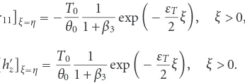
The displacement and temperature in the solid are both continuous at the elastic wave front while the stress and the perturbed magnetic field suffer finite discontinuities at this location. The discontinuities decay exponentially with distance from the boundary. The solution (2.52) for perturbed field in vacuum represents a wave propagating with Alfv’en acoustic wave 1/βwithout any attenuation. Further, the perturbed field in vacuum is con-tinuous at Alfv’en acoustic wave front. The finite discontinuities of the stress field and the perturbed magnetic field at the elastic wave front in the solid are not constants and are given by
σ11ξ=η= −T0
θ0 1 1 +β3exp
−εT
2 ξ
, ξ >0,
hz
ξ=η=
T0 θ0
1 1 +β3exp
−εT
2 ξ
, ξ >0.
(3.1)
With an aim to illustrate the problem, we will present some numerical results. We have chosen a copper-like material for whichεT=0.0168,β3=0.05. We takeCT=2.
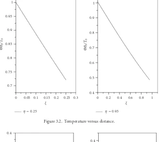
Using this data, the values of the physical quantities are evaluated as plotted in Figures 3.1,3.2,3.3, and3.4.
0.7 0.75 0.8 0.85 0.9 0.95 1
Θ
θ0 /T0
0 0.05 0.1 0.15 0.2 0.25 0.3
ξ
η=0.25
0.4 0.5 0.6 0.7 0.8 0.9 1
Θ
θ0
/T
0
0 0.2 0.4 0.6 0.8 1
ξ
[image:14.468.71.398.84.377.2]η=0.95
Figure 3.2. Temperature versus distance.
−1
−0.8
−0.6
−0.4
−0.2
0 0.2 0.4
hz /θ0 /T0
0 0.05 0.1 0.15 0.2 0.25 0.3
ξ η=0.25
−0.8
−0.6
−0.4
−0.2
0 0.2 0.4
hz /θ0 /T0
0 0.2 0.4 0.6 0.8 1
[image:14.468.69.394.344.605.2]ξ η=0.95
−1
−0.8
−0.6
−0.4
−0.2
0 0.2
σ11 θ0 /T0
0 0.05 0.1 0.15 0.2 0.25 0.3
ξ η=0.25
−0.8
−0.6
−0.4
−0.2
0 0.2 0.4
σ11 θ0 /T0
0 0.2 0.4 0.6 0.8 1
[image:15.468.63.401.65.422.2]ξ η=0.95
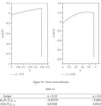
Figure 3.4. Stress versus distance.
Table 3.1
Jumps η=0.25 η=0.95
[σ11θ0/T0]ξ=η −0.95170 −0.94889
[hzθ0/T0]ξ=η 0.95298 0.95032
forη=0.25 and in the range 0< ξ <0.622 forη=0.95, which means that it is in opposite direction.
Figure 3.2indicates variation of temperature versus distance. The values of tempera-ture gradually decrease with distanceξ, the curve is continuous in agreement with the theoretical results.
Figure 3.3shows that the perturbed field gradually increases with distance for small timeη=0.25 and suffers a finite jump at the elastic wave frontξ=η=0.25. Further for timeη=0.95, the value of perturbed field first gradually increases with distance and then again it gradually decreases and suffers a finite jump at the elastic wave frontξ=η=0.95. Figure 3.4gives the stress distribution. Stress curve suffers a finite jump at two instants η=0.25 andη=0.95, where the wave front is positioned at the two instantsη=0.25 and η=0.95 in agreement with theoretical results.
Finite jumps in stress and the perturbed magnetic fields at two different instantsη=
0.25 andη=0.95 are exhibited inTable 3.1.
Acknowledgment
The authors thank the respected reviewers for their valuable suggestions.
References
[1] H. S. Carslaw and J. C. Jaeger,Conduction of Heat in Solids, 2nd ed., Clarendon Press, Oxford, 1959.
[2] D. Chand, J. N. Sharma, and S. P. Sud,Transient generalised magneto-thermo-elastic waves in a rotating half-space, Internat. J. Engrg. Sci.28(1990), no. 6, 547–556.
[3] G. Chatterjee (Roy) and S. K. Roychoudhuri,The coupled magneto-thermo-elastic problem in elastic half-space with two relaxation times, Internat. J. Engrg. Sci.23(1985), no. 9, 975– 986.
[4] A. E. Green and K. A. Lindsay,Thermo-elasticity, J. Elasticity2(1972), 1–7.
[5] A. E. Green and P. M. Naghdi,On undamped heat sources in an elastic solid, J. Thermal Stresses 15(1992), 253–264.
[6] ,Thermoelasticity without energy dissipation, J. Elasticity31(1993), no. 3, 189–208. [7] S. Kaliski and W. Nowacki,Combined elastic and electromagnetic waves produced by thermal
shock in the case of a medium of finite electric conductivity, Bull. Acad. Polon. Sci. S´er. Sci. Tech. , 1,10(1962), 213–223.
[8] H. W. Lord and Y. Shulman,A generalized dynamical theory of thermoelasticity, J. Mech. Phys. Solids15(1967), 299–309.
[9] C. Massalas and A. Dalamangas,Coupled magneto-thermo-elastic problem in elastic half-space, Internat. J. Engrg. Sci.21(1983), no. 2, 171–178.
[10] ,Coupled magnetothermoelastic problem in elastic half-space having finite conductivity, Internat. J. Engrg. Sci.21(1983), no. 8, 991–999.
[11] W. Nowacki,Dynamical Problems of thermo-elasticity, Nordhoff, Layden, 1975.
[12] S. K. Roychoudhuri,Electro-magneto-thermo-elastic plane waves in rotating media with thermal relaxation, Internat. J. Engrg. Sci.22(1984), no. 5, 519–530.
[13] , On magneto-thermo-elastic plane waves in infinite rotating media with thermal re-laxation, Proc. IUTAM Symposium on “Electro-Magneto-Mechanical Interactions in De-formable Solids and Structures” (Y. Yamamoto and K. Miya, eds.), Elsevier, North Holland, 1986, pp. 361–366.
[14] S. K. Roychoudhuri and S. Banerjee,Magneto-thermo-elastic waves induced by a thermal shock in a finitely conducting elastic half space, Int. J. Math. Math. Sci.19(1996), no. 1, 131–143. [15] S. K. Roychoudhuri and G. Chatterjee (Roy),A coupled magneto-thermoelastic problem in a
perfectly conducting elastic half-space with thermal relaxation, Int. J. Math. Math. Sci.13 (1990), no. 3, 567–578.
[16] ,Temperature-rate dependent magneto- thermo-elastic waves in a finitely conducting elas-tic half-space, Comput. Math. Appl.19(1990), no. 5, 85–93.
[17] S. K. Roychoudhuri and L. Debnath,Magneto-thermo-elastic plane waves in rotating media, Internat. J. Engrg. Sci.21(1983), no. 2, 155–163.
S. K. Roychoudhuri: Department of Mathematics, University of Burdwan, Bardhaman 713104, West Bengal, India
E-mail address:skrc bu [email protected]
Nupur Bandyopadhyay: Department of Mathematics, University of Burdwan, Bardhaman 713104, West Bengal, India