Observing Tool Bit Conditions in Turning Process
through OpenCV Programming Function
Ahmad Yusairi Bani Hashim*, Muhammad Amirul Amin Suaadi
Department of Robotics and Automation, Faculty of Manufacturing Engineering, Technical University of Malaysia Malacca, Melaka, Malaysia
Copyright©2017 by authors, all rights reserved. Authors agree that this article remains permanently open access under the terms of the Creative Commons Attribution License 4.0 International License
Abstract
Machine vision provides flexibility and further automation options to manufacturers. It helps detect product defects, complete a different number of tasks efficiently. The goal of this work was to develop a machine vision program that would monitor the state of the tool bit state and signals it through a software pop-up when the tool bit exhibited anomaly while cutting. The program would sense when the tool bit shows an anomaly of its sharpness while cutting. Canny algorithm and thresholding were the techniques to perform video analysis. Canny edge detector algorithm was used to change the RGB image to a grayscale-based image. The image would display only the object’s edges so that the tool bit’s sharp edge was visible and was analyzable for tool wear condition. The monitoring of the tool wear condition using OpenCV programming functions was proven workable. Further codes enhancements are needed to provide an effective program and to produce reliable results.Keywords
Tool Bit, Turning Process, Tool Wear, OpenCV, Canny Edge Detector, Python1. Introduction
Machine vision provides flexibility and further automation options to manufacturers. It helps detect product defects, complete a different number of tasks efficiently. The metal cutting operation, on the other hand, is a typical process found in manufacturing industries. Besides being essential to the production process, metal cutting is likewise a finishing operation used to accomplish a high dimensional in term of accuracy and almost to the desired surface finish [1].
Conventional metal cutting processes are milling, boring, turning, grinding and drilling. These cutting procedures are dependent on skilled workers until automated machining started to substitute human operators with mechanized machining processes. Computerized machining caught
manufacturer’s attention who were considering to reduce production cost while increasing profit. They saw that automated metal cutting processes could replace a human worker, increase profitability, reduce production costs, and upgrade product quality [2], [3], [4].
A lathe is a machining instrument that does sanding, knurling, facing, cutting, deformation or drilling, turning. The tool bit determines the finished product a perfect work piece. High carbon tool steels constitute all tool bits with the proper hardening and tempering. High-speed steel (HSS), ceramic and diamond, sintered carbide are examples of tool materials used on cutting application.
Monitoring tool wear is a region of active research. Tool condition plays an important role that affects the surface finish, in addition to, the dimensional integrity of the workpiece and vibration in the tool itself. Besides, a robust tool wear monitoring system can decrease machine downtime brought on by changing the tool to get fewer process interruptions.
The data obtained from the tool wear monitoring system can be utilized for a few purposes, including the foundation of tool change arrangement, financial optimization of the machining operation, online process control to make up for tool wear, and, in some cases, the prevention of catastrophic tool failure.
In getting higher productivity, it is necessary to plan for manufacturing and computer aided processes [5]. Optimizing machining parameters such as feed rate, cutting speed and the depth of cut would minimize tool wear, thus improving machinability.
2. Background
2.1. Turning Process
Cutting in machining remove material from the surface of a workpiece by producing chips [6]. In a conventional lathe, the machine operator checks the measurements routinely to get perfect accuracy. It is critical because of the high chances that the operator would expel abundance metal from the workpiece. Therefore, the entire workpiece will be a wasted, hence loss of money and time. The final geometry is achieved when the necessary part of the workpiece has been eliminated.
The purpose of machining is to accomplish a finished product of the desired dimension, shape and surface roughness quality. Machining is smooth when a sharp cutting tool is used to eradicate some parts of the material and leave the needed part in final form. In a turning process, there are three critical parameters: cutting speed, depth of cut and feed rate. A little feed rate would yield a small surface roughness. A finished surface roughness is determined by the feed rate, in combination with other parameter settings [7].
It is important to choose a proper the cutting parameters for a given cutting tool-workpiece material and machine tool for successful implementation of hard turning [8]. In fact, the feed rate is the most important factor that influences the generation of surface roughness [9]. The spindle speed contributes 63.90%, depth of cut contributes only 11.32%, and feed rate contributes at least 8.33% for a surface roughness [10].
2.2. Image Processing
Image processing is about preparing of images by mathematical operations. The pictures may come in the forms of videos or still images. The typical method in image processing is treating the image as a two-dimensional signal by applying a signal processing technique. The primary goal of a machine vision, on the other hand, is to build a model of the real world from images. It improves useful information based on a scene from its two-dimensional projections.
All images are two-dimensional projections of the three-dimensional world. Therefore, the information that the image carries needs improvement. This recovery requires the inversion of a many-to-one mapping [11]. By enhancing the images, some information may be retrieved from them.
Computer vision aims to replicate the effect of human vision by electronically observation and to read a picture. Dynamic scenes such as moving object or a moving camera, are increasingly common and symbolize another way of making computer vision more complicated [12, 13].
Binary images can take on two values, which are typical “0” and 1, or black and white. It is referred to as a 1-bit per pixel image because it takes only one binary digit to represent each pixel. Usually, these types of images are
mostly used in computer vision applications. The only information needed for the task is general shape or outline information. This kind of images is frequently created from gray-scale images through a threshold operation. A threshold operation will make every pixel above the threshold value turns white (“1”), and those below it turns black (“0”). Even though in this operation a lot of information is missing, the resulting image file is much smaller, thus making it easier to store and transmit.
Gray-scale images are monochrome, or one color, images. These images contain only brightness information with no color information. The number of different brightness levels available can be determined by the number of bits used for each pixel. The standard image comprehends 8-bit per pixel data allows a 256 level that is from 0 to 255 different brightness levels. The 8-bit representation matches to 8-bits of data. It is the average small unit in the world of digital computers [14].
A brightness histogram ℎ(𝑧) of an image offers the frequency of the brightness value of 𝑧. A histogram of an image with 𝐿 gray-levels is symbolized by a one-dimensional array with 𝐿 elements. Histogram is the only complete information about the image that is accessible. Histogram is used when it comes to finding optimal illumination conditions for catching an image, gray-scale transformations, and image division to object and background. A histogram may produce specific images, explanation, a transform of the object located on a continuous background [12].
After images are converted to grayscale, they may contain unequally distributed gray values. The images, in which all intensity values that lie within a small range, are commonly found as the reduced contrast images. Histogram equalization is a technique for extending the contrast of such images by consistently rearranging the gray values. Histogram modification improves the quality of a picture that is useful when the image is formed from the rational view. Histogram equalization enhances the contrast by plotting the gray values to estimation to a uniform scattering.
A histogram is studied to select the suitable threshold value. A histogram of an image is a plot of gray level versus the number of pixels in the picture at every gray level. A threshold is experimentally selected that will separate the object from the background based on the values found at the peaks and the valleys of the histogram. A simple technique of spontaneously searching a threshold is by running an iterative process. This technique is the isodata method that applies the 𝑘-means clustering algorithm used in pattern recognition to divide two clusters [14].
setting all values upper the specified gray level to “1”, and all values lower or equal to the specified value to “0”. The real values for the “0” and “1” can be anything. It is 255 that is usually transformed to a “1,” and 0 is utilized for a “0”. The “0” will appear black, and “1” white.
The initial phase of vision processing recognizes features in images. The features are related to the properties and the structure of objects in a scene. One of the features is the edges. Edges usually occur on the boundary between two different regions in images. Edge detection is commonly used to recover the information from pictures [11].
The line detection process applies the edge detection methods. It is, however, difficult to identify object boundaries by marking potential edge points. The potential edge points corresponding to the places in an image where rapid changes in term of brightness occur [14]. Edge detectors are essential local image pre-processing methods used to locate changes in the intensity function of a picture. These methods are useful particularly if the edges are pixels, in term of, brightness that have turned sharply [12].
2.3. Operators
Roberts operator is one of the oldest of its kind. It is effortless to calculate as it uses only a 2 by 2 neighborhood of the current pixel. The operator’s masks, 𝐺𝑥 and 𝐺𝑦 are defined in (1). The magnitude of the edge is calculated as (2). The major disadvantage of this operator is its high sensitivity towards noise due to very few pixels are used to estimate the gradient.
|𝐺𝑥| =�+10 −01�,�𝐺𝑦�=�−01 +10 � (1) |𝐺| = |𝐺𝑥| +�𝐺𝑦� (2) Laplacian is an operator that provides edge magnitude only. The Laplacian equation is approached in digital images by a convolution sum. A mask, ℎ of a 3 by 3 for a 4-neighborhood and an 8-neighborhood is defined in (3), respectively.
ℎ=�01 −14 10
0 1 0�,ℎ=�
1 1 1
1 −8 1
1 1 1� (3)
Laplacian operator, defined in (4), with the stressed significance of the dominant pixel or its neighborhood is occasionally used. In this estimation, it loses invariance to the rotation. Unfortunately, Laplacian operation reacts extra to some edges in the image.
ℎ=�−21 −−14 −21
2 −1 2 �,ℎ=�
−1 2 −1
2 −4 2
−1 2 −1� (4) Sobel operator is used as a simple detector of horizontality and verticality of edges, ℎ1 and ℎ2 can be implemented using convolution masks, defined in (5).
ℎ1=�
1 2 1
0 0 0
−1 −2 −1�,ℎ2=�
−1 0 1
−2 0 2
−1 0 1� (5) If ℎ1 returns 𝑦 and ℎ2 returns 𝑥, thus, the magnitude or the edge strength, 𝑀 can be calculated and derived using (6), while the direction is defined as tan−1(𝑦 𝑥⁄ ) [12].
𝑀=�𝑥2+𝑦2 or 𝑀= |𝑥| + |𝑦| (6) Prewitt operator uses the similar equations as the Sobel operator, apart from the constant 𝑐= 1, hence (7). Different from Sobel operator, Prewitt operator does not place any weight on pixels that are closer to the middle of the masks [11].
ℎ𝑥=�
−1 0 1
−1 0 1
−1 0 1�,ℎ𝑦=�
1 1 1
0 0 0
−1 −1 −1� (7) Canny Edge Detector or the Canny algorithm was proposed in 1986 [15]. It is based on a detailed mathematical model for finding edges [14]. The edge design is a step edge which is corrupted by Gaussian noise or white noise. The algorithm consists of four primary steps [16].
In the first step, it smoothes the image with a Gaussian filter. An array of smoothed data may be obtained from convolving the image with Gaussian smoothing filter using separable filtering where σ is the spread of the Gaussian and controls the degree of smoothing [11]. In the second step, by using similar equations to Sobel or Prewitt operators, the edge magnitude and the edge direction may be defined as (8) and (9), respectively [14].
Edge magnitude=�𝑐12+𝑐22 (8) Edge direction= tan−1�𝑐1
𝑐2� (9)
In the third step, non-maxima suppression to the gradient magnitude is applied. This action is necessary to verify if the edges found in an image are significant. An edge will be removed as a side point if it is found insignificant. The thick edges can also be thinner, by selecting the high point along a gradient direction [14].
In the final step, the double thresholding is applied to join sides once they have been detected. It will also remove the false responses. This technique is also known as hysteresis. Streaking may break up contours of the edges as the operator oscillates above and below the threshold. This can be removed by this last step which employing a high threshold and a lower limit. These thresholds that are high and low are set based on the estimation of signal-to-noise ratio [12].
2.4. OpenCV
In 2005, OpenCV was utilized on Stanley, the vehicle which won 2005 DARPA Grand Challenge. Its progressive improvement proceeded under the support of Willow Garage, with Gary Bradsky and Vadim Pisarevsky driving the venture.
Now, OpenCV supports a considerable measure of calculations or algorithms identified with computer vision and machine learning. OpenCV augments a wide assortment of programming dialects such as C++, Python, and Java. It is accessible on various operating systems including Windows, Linux, OS X, Android, and iOS. The SimpleCV is a derivative of OpenCV offers a simple approach to coding. It reduces the complexity of programming that is found sufficient for a rapid prototyping of a vision system [18].
Interfaces given CUDA and OpenCL are additionally under dynamic improvement for fast GPU operations. OpenCV-Python is the Python API of OpenCV. It is the distinct characteristics of OpenCV C++ API and Python scripting language.
There are a couple of important OpenCV tools or library useful in image and video analyses such as NumPy and Scipy. NumPy includes bolstering for massive multidimensional clusters and grids to Python.
It comprises of an extensive library of high-level numerical capacities to work in these groups. On OpenCV, pictures are read in as NumPy clusters. Other mathematical, image handling and machine learning libraries are based on top of NumPy.
SciPy is a capable, logical library based on top of NumPy. It is sub-bundles incorporate, for example, 𝑙𝑖𝑛𝑎𝑙𝑔 (linear algebra), 𝑜𝑝𝑡𝑖𝑚𝑖𝑧𝑒 (enhancement and root-discovering schedules), 𝑠𝑡𝑎𝑡𝑠 (measurable distributions and capacities),
𝑛𝑑𝑖𝑚𝑎𝑔𝑒 (n-dimensional picture processing),
𝑖𝑛𝑡𝑒𝑟𝑝𝑜𝑙𝑎𝑡𝑒 (interpolation and smoothing splines),
𝑓𝑓𝑡𝑝𝑎𝑐𝑘 (Fast Fourier Transform schedules), 𝑐𝑙𝑢𝑠𝑡𝑒𝑟
(clustering calculations).
OpenCV was chosen to analyze videos for the following
reasons: 1) It provides open source programming functions, 2) it allows programming flexibility as the users may amend the existing codes when necessary, and 3) this work was designed to avoid expensive licensed tools by implementing the algorithms in Python environment.
3. Experimental Setup
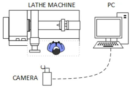
[image:4.595.323.536.340.487.2]Figure 1 shows the experimental setup. A lathe machine was used to perform the straight turning operation using a single-point tool bit of HSS or carbide to cut the workpieces. A web camera (Logitech 1080p) was utilized to record the cutting event. The recorded video was processed to extract the relevant information using OpenCV. The video data was kept in computer storage. The Python programming platform and OpenCV programming functions were the computing tools applied for the video analysis. Figure 2 depicts the program flow chart where OpenCV programming functions were used in Python environment.
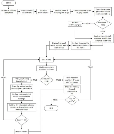
Figure 2. The program flow chart where OpenCV programming functions were used in Python environment. There are a couple of phrases that might not be familiar to the readers such as “Tajam” means sharp, “Tumpul” means blunt.
The functions such as 𝑎𝑏𝑠𝑑𝑖𝑓𝑓, 𝑏𝑜𝑢𝑛𝑑𝑖𝑛𝑔𝑅𝑒𝑐𝑡, and
𝐹𝑟𝑎𝑚𝑒𝐷𝑒𝑙𝑡𝑎 were applied to compute the video frames while the scene was being recorded.
The experiment was divided into four phases: capturing the data or image, export the data to OpenCV, process and analyze the data by using Canny Edge Detector, and lastly was the tool wear analysis. The analyses were done, firstly,
by data processing and manipulating. All the information in the form of images was collected and was then saved in a computer.
undergo filtering to remove noise. Since the contrast was poor, performing histogram equalization was necessary.
The next phase followed by filtering algorithm using the 3 by 3 Gaussian. In order to determine whether the tool was used or unused, the master or the original image of the unworn tool was set to find a threshold value. It was compared with a subsequent image from the video. Canny edge detector was utilized where the threshold value must be in binary in order to execute the algorithm. The operator would compare pixel-to-pixel between the image, and it would return a zero (0) if the pixel was identical otherwise it would return a one (1) if the pixel was not equal [19].
The function 𝑐𝑣2.𝑡ℎ𝑟𝑒𝑠ℎ𝑜𝑙𝑑 checked each pixel value. If the function found a pixel that had a value larger than a threshold value then it would assign a unique value to the pixel. The first argument was the source image that had been converted to a grayscale image. The second argument was the threshold value used to classify the pixel values. The third argument was the 𝑚𝑎𝑥𝑉𝑎𝑙 , that represented the value to be given if the pixel value was, more than or sometimes less than, the threshold value.
OpenCV provides different styles of thresholding, and it is decided by the fourth parameter of the function. It puts all the arguments in a single function that is 𝑐𝑣2.𝐶𝑎𝑛𝑛𝑦(). The first argument is the input image. The second arguments are 𝑚𝑖𝑛𝑉𝑎𝑙 and 𝑚𝑎𝑥𝑉𝑎𝑙. The third argument is 𝑎𝑝𝑒𝑟𝑡𝑢𝑟𝑒_𝑠𝑖𝑧𝑒. It is the size of Sobel kernel used for find image gradients, is by default equals to 3. The last argument is 𝐿2𝑔𝑟𝑎𝑑𝑖𝑒𝑛𝑡 that specifies the equation for finding gradient magnitude. If its status is true then it would apply (1), otherwise (2). The function is by default, False.
4. Results and Discussion
The key feature of image processing is to characterize the sharpness of the tool bit. The tool bit's sharpness, however, is not easily described. It requires algorithm amendments and adjustments before the results reach to some degrees of validity.
The factors of interference ranging from the lighting issues, the distorted and incoherent chips from the workpiece, an unknown tool bit's edge location, and the camera placement. As the camera produced analog data, enhancing the triggering values with time delayed would provide good results.
[image:6.595.313.551.79.236.2]Figure 3 shows a raw image was initially taken before the cutting process began. The tool was initially sharp. The image was assigned as the reference image. It would be compared to when analyzing the state of the tool bit. Figure 4, on the other hand, shows three separate real-time streamings of the pure, grayscale, and Canny image, respectively.
[image:6.595.313.551.297.461.2]Figure 3. The initial image prior to cutting. The tool bit was sharp enough to cut the workpiece. The image would be used as the reference image for analysis. The algorithm, however, was not programmed to analyze the workpiece’s surface roughness.
Figure 4. A real-time view of pure, gray-scale, and Canny image streamings while the turning and cutting operations were in progress. While cutting, some of the chips might block the view of the targeted point, which was the tooltip. At that time, the program might not be able to detect if the sharp tip had become dull. However, when the machine operator retracted the tool, the program would immediately process the image and identify the flaw.
The Canny algorithm makes edge detection possible. Table 1 lists the code that realized Canny on Python scripting language. It applied a Gaussian filter to smooth the image and to reduce the noises, which later found the gradient intensities.
Table 1. The code that realized the Canny algorithm.
thresh = cv2.Canny(frame,100,200)
(_,cnts,_) =
After using suppression to get rid of spurious response to the edge detection, a second threshold was applied to determine all possible edges. The edges were a track with hysteresis and drawn to another frame stream as shown in Figure 5. The “Mata Alat: Tumpul” is literally translated to “Tool bit: Blunt.”
Figure 5. A Canny image view when some degrees of tool bit bluntness were sensed.
From Table 1, the “frame” was the variable that was declared for the Canny frame itself. It originated from the RGB frame that was converted to grayscale. The second and third arguments were the value of 100 and 200. These were the 𝑚𝑖𝑛𝑉𝑎𝑙 and 𝑚𝑎𝑥𝑉𝑎𝑙, respectively. These two values would determine if the correct results were to be obtained.
Apart from detecting the edges of an image, one more important issue involving Canny edge detection is that there are always changes to analog data. It varies from the light intensity and the moving object. In order to analyze the whole frame changes, the delta method was used. It computed an image frame that varied by time, providing immediate changes in grayscale intensity. The frames could be observed in real-time. Figure 6 shows the delta image. The command line for delta frame is provided in Table 2.
The delta image began to work as the first frame was captured and defined as the starting frame, represented by an initializing frame. The latest frame became the second frame that was virtually stacked over the initializing frame so that changes in grayscale intensity could be clearly observed.
[image:7.595.313.551.79.255.2]The intensity of the tool bit was evident when the camera was initialized. The tool bit state of sharpness was observed. After getting the frames of Canny and the delta images, the thresholding process took place. The thresholding was the process of image segmentation, and in this contexts, it would differentiate the foreground and the background colors. The output would be in the binary image with white or black pixels.
[image:7.595.58.297.155.318.2]Figure 6. The delta image view. The view was purposely computed to produce such a blurry picture.
Table 2. The code used to realize the delta image algorithm. The instructions were given to find the difference between the latest and the previous images. The image was in the form of a frame that was converted to a grayscale image.
# Kira perbezaan antara bingkai lama dengan bingkai baharu frameDelta = cv2.absdiff(firstFrame,gray)
The thresholding value was then compared to each frame to determine the step difference between the sharp state and blunt state. This step was important to ascertain the sharpness of the tool bit. When the captured frame became binary, it increased the processing speed. As a result, the convergence rate increased thus the final results would be shown on the text display.
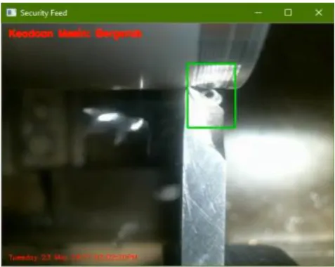
The code for threshold and bounding rectangle is given in Table 3. The contour would be drawn in a green box. It could be seen when the machine state was in motion as illustrated in Figure 7. The drawn outline would stick at the tool’s tip where the chips were seen flew off.
Table 3. The code that realized the threshold and the green contour.
(x,y,w,h) = cv2.boundingRect(c)
cv2.rectangle(frame,(x,y), (x+w,y+h),(0,255,0),2) text = "Bergerak"
# Mulakan bawah koordinate ambang untuk dapatkan perbezaan warna
color = int(thresh[240,190]) if color == 0:
Figure 7. A green contour was marked to enclose the sharp edge area. The image was cropped from a video while in the analysis mode that was the reason behind the low-quality image.
The most important part was the program itself that stored the state of the first frame when the Python program started. It set an initial value where the threshold and delta frame obtained the initials readings. A loop was placed to find the moving objects that were detected from the delta frame and to draw the contour. The chips were one of the primary objects identified as the minimum area of detection was programmed below 50.
The focus level of the camera itself was another important issue. There was a distant gap between the tool and the webcam. The Logitech 1080p used in this work was able to record the view efficiently. A Python code was executed to disable autofocus on the camera, and the webcam was manually focused by using its own software to detect the edges perfectly.
5. Conclusions
Tool bit sharpness plays an essential role in order to get an excellent surface roughness that influences the smoothness of the machined workpiece. Moreover, it also improves the accuracy of the machining that will produce a correct dimension of the workpiece. OpenCV provides with ready-made features that are compiled into a simple syntax that will generally reduce the length of the code. In addition, OpenCV is designed to work on all platforms, making it very portable to convert into different machines.
Out of various libraries, this work chose to utilize the OpenCV library. It functioned well for a real-time video processing. Data management was a major factor that controlled the speed and equalization of the results. Canny algorithm and thresholding were the techniques applied to perform video analysis. Canny edge detector algorithm was used to change the RGB image to a grayscale-based image. The image would display only the object’s edges so that the tool bit’s sharp edge was visible and was analyzable for tool
wear condition.
The innovation found in this work was the use of specific image processing operators such as the Canny operator in the OpenCV programming function. The approach to video analysis in this work differs from others. In the previous literature, similar works were found using licensed tools such as Matlab. Although there is research that applies open source codes for image analysis, this work adds to the existing list. In general, this work offers ideas to the general readers of an alternative to video processing using open source codes that will reduce dependency to expensive tools.
The monitoring of the tool wear condition using OpenCV programming functions was proven workable. Further scripts enhancements are needed to provide an effective program and to produce reliable results.
REFERENCES
[1] N. Singh, Systems approach to computer-integrated design and manufacturing: John Wiley & Sons, Inc., 1995.
[2] G. O’Donnell, P. Young, K. Kelly, and G. Byrne, "Towards the improvement of tool condition monitoring systems in the manufacturing environment," Journal of Materials Processing Technology, vol. 119, pp. 133-139, 2001.
[3] K. S. Park and S. H. Kim, "Artificial intelligence approaches to determination of CNC machining parameters in manufacturing: a review," Artificial Intelligence in Engineering, vol. 12, pp. 127-134, 1998.
[4] S. Purushothaman and Y. Srinivasa, "A back-propagation algorithm applied to tool wear monitoring," International Journal of Machine Tools and Manufacture, vol. 34, pp. 625-631, 1994.
[5] S. Ali and N. Dhar, "Tool wear and surface roughness prediction using an artificial neural network (ANN) in turning steel under minimum quantity lubrication (MQL)," World Academy of Science, Engineering and Technology, vol. 62, pp. 830-839, 2010.
[6] S. Kalpakjian, S. R. Schmid, and H. Musa, Manufacturing engineering and technology: machining: China Machine Press, 2011.
[7] E. D. Kirby, "A parameter design study in a turning operation using the Taguchi method," The technology interface, pp. 1-14, 2006.
[8] A. Narasimhulu, S. Ghosh, and P. Rao, "Study of Tool Wear Mechanisms and Mathematical Modeling of Flank Wear During Machining of Ti Alloy (Ti6Al4V)," Journal of The Institution of Engineers (India): Series C, vol. 96, pp. 279-285, 2015.
[9] M. R. Reddy, P. R. Kumar, and G. K. M. Rao, "Effect of feed rate on the generation of surface roughness in turning," International Journal of Engineering Science and Technology (IJEST), vol. 3, 2011.
parameters on MRR and surface roughness in turning EN-8," Current Trends in Engineering Research, vol. 1, 2011.
[11]R. Jain, R. Kasturi, and B. G. Schunck, Machine vision vol. 5: McGraw-Hill New York, 1995.
[12]M. Sonka, V. Hlavac, and R. Boyle, Image processing, analysis, and machine vision: Cengage Learning, 2014. [13]N. S. A. Ramdan, A. Y. B. Hashim, S. R. Kamat, and S. A.
Asmai, "Comparison on Techniques for Multiple Video Streaming via Webcam for Manufacturing Engineering Purpose," Applied Mechanics and Materials, vol. 761, pp. 116-119, 2015.
[14]S. E. Umbaugh, Digital image processing and analysis: human and computer vision applications with CVIPtools: CRC press, 2016.
[15]J. Canny, "A computational approach to edge detection," IEEE
Transactions on pattern analysis and machine intelligence, pp. 679-698, 1986.
[16]R. Deriche, "Using Canny's criteria to derive a recursively implemented optimal edge detector," International journal of computer vision, vol. 1, pp. 167-187, 1987.
[17]A. Mordvintsev and K. Abid, "Opencv-python tutorials documentation," Obtenido de https://media. readthedocs. org/pdf/opencv-python-tutroals/latest/opencv-python-tutroals. pdf, 2014.
[18]N. S. A. Ramdan, A. Y. Bani Hashim, S. R. Kamat, and S. A. Asmai, "Detecting human movement by image histogram to monitor body discomfort," International Journal of Imaging and Robotics, 2016 2016.