ADESHINA ADEKUNLE MICHEAL
A thesis submitted in
fulfilment of the requirement for the award of the Doctor of Philosophy
Faculty of Computer Science and Information Technology Universiti Tun Hussein Onn Malaysia
ABSTRACT
ABSTRAK
CONTENTS
TITLE i
DECLARATION ii
DEDICATION iii
ACKNOWLEDGMENT iv
ABSTRACT v
LIST OF PUBLICATIONS vii
CONTENTS ix
LIST OF TABLES xiv
LIST OF FIGURES xv
LIST OF SYMBOLS AND ABBREVIATIONS xix
LIST OF APPENDICES xxiv
CHAPTER 1 INTRODUCTION 1.1 Background Study 1
1.2 Brain Anatomy and Abnormalities 2
1.3 Motivation 4
1.4 Research Questions 7
1.5 Research Objectives 7
1.6 Scope of the Research 8
CHAPTER 2 VISUALIZATION OF VOLUMETRIC DATASETS
2.1 Introduction 10
2.2 Volume Visualization 12
2.3 Volumetric Image Datasets 13
2.4 Medical Imaging Modalities 16
2.4.1 Computed Tomography 17
2.4.2 Magnetic Resonance Imaging 18
2.4.3 Clinical Applications / Relevancies 20
2.5 Dataset Pre-Processing Techniques 21
2.5.1 Filtering, Enhancement, Detection& Extraction 21
2.5.2 Volume Segmentation 23
2.5.3 Data Reduction 25
2.6 Medical Volume Visualization 26
2.6.1 Volumetric Image Visualization 27
2.6.2 Multiplanar Reformation (MPR) 28
2.6.3 Surface Rendering Technique 29
2.6.4 Direct Rendering Technique 30
2.6.5 3-D Reconstruction 31
2.7 CUDA Technology 32
2.8 Software Components 36
2.8.1 Graphics Execution 37
2.8.2 Volume Rendering 39
2.8.2.1 Classification 40
2.8.2.2 Rendering 42
2.9 Frameworks in Medical Volume Visualization 43
2.9.1 Probe-Volume: An Exploratory Volume 45
Visualization Framework 2.9.2 VDVR: Verifiable Visualization of 46
2.9.3 GPU Accelerated Generation of Digitally 48
Reconstructed Radiographs for 2-D / 3-D Image Registration 2.9.4 Volume Visualization with Grid-Independent 48
Adaptive Monte Carlo Sampling 2.9.5 Framework for Volume Segmentation, 49
Visualization using Augmented Reality 2.9.6 Illustrative Volume Visualization using GPU- 50
Based Particle Systems 2.9.7 Volumetric Ambient Occlusion for Real-Time 51
Rendering and Games 2.9.8 An Improved Volume Rendering Algorithm 52
Based on Voxel Segmentation 2.9.9 ParaView Visualization Framework 53
2.9.10 VolView Framework 54
2.10 Advantages & Disadvantages of Previous Frameworks 55
2.11 Summary 59
CHAPTER 3 METHODOLOGY: THE DEVELOPMENT OF SurLens 3.1 Introduction 62
3.2 SurLens Architecture 63
3.3 The Framework of SurLens 65
3.3.1 Datasets Pre-Processing 68
3.3.1.1 Application of Projective Plane Theorem 68 3.3.1.2 Coordinates Systems 74
3.3.1.3 Intensity Matching 81
3.3.2 Accelerating Hardware 83
3.3.2.1 Data Structuring & Fragmentation 85
3.3.4 Volume Rendering Phase 90
3.3.4.1 Camera Model 91
3.3.4.2 Volume Classification 93
3.3.4.3 Shading and Gradient Computation 95
3.3.4.4 Interpolation / Re-sampling 97
3.3.4.5 Compositing 98
3.4 Summary 102
CHAPTER 4 IMPLEMENTATION AND TEST DATASETS 4.1 Introduction 104
4.2 Conversion Scheme 108
4.3 Feature & Edge Detection Scheme 112
4.4 Automatic Feature & Mapping Technique 115
4.5 SurLens Robust Algorithms’ for Mass data 119
4.6 Summary 120
CHAPTER 5 RESULTS AND DISCUSSION 5.1 Introduction 122
5.2 Results of New Feature & Edge Detection Scheme 123
5.2.1 Experimentation with MRA Datasets 124
5.2.2 Experimentation with DTI Datasets 126
5.2.3 Experimentation with T1-FLASH Datasets 128
5.2.4 Experimentation with T1-MPRAGE Datasets 129
5.3 Results of New Feature Mapping Techniques 130
5.3.1 Experimentation with MRA Datasets 131
5.3.2 Experimentation with DTI Datasets 142
5.3.3 Experimentation with T1-FLASH Datasets 145
5.3.4 Experimentation with T1-MPRAGE Datasets 147
5.4.1 ParaView & VolView Visualization Systems 149
5.5 Results of Robust Algorithms for Mass data 154
5.5.1 Speed Evaluation with MRA Datasets 155
5.5.2 Speed Evaluation with DTI Datasets 159
5.5.3 Speed Evaluation with T1-FLASH Dataset 160
5.5.4 Speed Evaluation with T1-MPRAGE Dataset 161
5.6 Summary 162
CHAPTER 6 CONCLUSION 6.1. Introduction 164
6.2. Conclusion 165
6.3. Contributions 169
6.4. Future Works 170
REFERENCES 171
APPENDIX A 195
APPENDIX B 214
LIST OF TABLES
2.1 Comparison of CPU and GPU 32
3.1 Homogeneous Coordinates Representation of Points and Lines 73
3.2 SurLens Access Design to Intensity 82
4.1 Experimental Testbeds 107
5.1 MRA Speed Evaluation for Datasets of Patient_001 to Patient_009 155
5.2 MRA Speed Evaluation for Datasets of Patient_010 to Patient_015 156
5.3 MRA Speed Evaluation for Datasets of Patient_016 to Patient_020 157
5.4 Randomly Selected Patients MRA Datasets for Speed Evaluation 158
5.5 Speed Evaluation for Selected Patients DTI Datasets 159
5.6 Speed Evaluation for Selected Patients T1-FLASH Datasets 160
LIST OF FIGURES
1.1 Conventional pathologists’ slides viewing microscope 5
1.2 Clinical support with visualization 5
2.1 Volumetric Data in Cartesian Grid 15
2.2 Data Structure Grids 16
2.3 An example of a CT slice, a head scan 18
2.4 An example of an MRI slice, brain’s Scan 20
2.5 VDVR Pipeline 47
2.6 The GPGPU Paradigm 50
3.1 SurLens Architecture 64
3.2 SurLens Framework Overview 66
3.3 SurLens Framework Phases 67
3.4 Parallel Lines in Projective Plane 69
3.5 Point Estimation of 2-D Slices 70
3.6 Translation 75
3.7 Scaling about the Origin 77
3.8 Rotation about x-axis 77
3.9 Rotation about y-axis 78
3.10 Rotation about z-axis 79
3.11 Algorithm1: SurLens Algorithm for Dataset Pre-Processing 81
3.12 Algorithm 2: SurLens Algorithm for Accelerating Hardware 82
3.13 SurLens-CUDA Architecture 84
3.14 SurLens Data Fragmentation Procedures 87
3.15 SurLens Memory System Architecture 88
3.16 SurLens Graphic Execution Phase (Phase 3) 89
3.17 Algorithm 3: SurLens Algorithm for Graphic Execution 89
3.18 SurLens Volume Rendering Phase (Phase 4) 91
3.20 Ambient Lighting 95
3.21 Diffuse Lighting 96
3.22 Specular Lighting 96
3.23 Absorption and Emission along Light Rays 100
3.24 Algorithm 4: SurLens Algorithm for Volume Rendering 102
4.1 SurLens Conversion Scheme 108
4.2 SurLens Conversion Scheme: Design Pipeline for Data Array Structure 109
4.3 SurLens Conversion Scheme: Design Pipeline for ImageData 110
4.4 SurLens Conversion Scheme: Design Pipeline of PointSet 111
4.5 Design of Contour Class for SurLens Feature & Edge Detection Scheme 112
4.6 Design of Anaglyph and Buffering Class for SurLens 113
Feature & Edge Detection Scheme 4.7 Overview of SurLens Automatic Feature Mapping Techniques 116
4.8-a SurLens Automatic Feature Mapping Techniques 116
4.8-b SurLens Automatic Feature Mapping Techniques 117
5.1-a Results of SurLens Feature & Edge Detection with MRA Datasets 124
5.1-b Results of SurLens Feature & Edge Detection with MRA Datasets 125
5.2-a Results of SurLens Feature & Edge Detection with DTI Datasets 126
5.2-b Results of SurLens Feature & Edge Detection with DTI Datasets 127
5.3-a Results of SurLens Feature & Edge Detection with T1-FLASH Datasets 128 5.3-b Results of SurLens Feature & Edge Detection with T1-FLASH Datasets 129 5.4-a Results of SurLens Feature & Edge Detection with 130
T1-MPRAGE Datasets 5.4-b Results of SurLens Feature & Edge Detection with 130
T1-MPRAGE Datasets 5.5 MRA Evaluation Datasets of Patient_001 and Patient_002 132
5.6. MRA Evaluation Datasets of Patient_003 and Patient_004 132
5.7. MRA Evaluation Datasets of Patient_005 133
5.8. MRA Evaluation Datasets of Patient_006 133
5.10. MRA Evaluation Datasets of Patient_010 135
5.11. MRA Evaluation Datasets of Patient_011 and Patient_013 135
5.12-a MRA Evaluation Datasets of Patient_014 and Patient_016 136
5.12-b MRA Evaluation Datasets of Patient_014 and Patient_016 136
5.13. MRA Evaluation Datasets of Patient_017 137
5.14 MRA Evaluation Datasets of Patient_018 and Patient_019 137
5.15. MRA Evaluation Datasets of Patient_020 and Patient_027 138
5.16. Randomly Selected Patient MRA Evaluation Datasets 138
5.17. MRA Evaluation Datasets of Patient_048 139
5.18. MRA Evaluation Datasets of Patient_052 and Patient_054 140
5.19. MRA Evaluation Datasets of Patient_061 and Patient_067 140
5.20-a. MRA Evaluation Datasets of Patient_073 140
5.20-b. MRA Evaluation Datasets of Patient_077 and Patient_083 141
5.21. MRA Evaluation Datasets of Patient_097 141
5.22. MRA Evaluation Datasets of Patient_098 142
5.23. DTI-Patient_067-Normal, Female, 57yrs 143
5.24. DTI-Patient_098-Abnormal, Female, 54yrs 143
5.25. DTI-Patient_054-Normal, Female, 34yrs 144
5.26. DTI-Patient_047-Abnormal, Female, 31yrs 144
5.27. T1-FLASH-Patient_067-Normal, Female, 57yrs 145
5.28. T1-FLASH-Patient_054-Normal, Female, 34yrs 145
5.29. T1-FLASH-Patient_047-Abnormal, Female, 31yrs 146
5.30. Patient_099-Stripped-FLASH (Normal Patient) 146
5.31. T1-MPRAGE-Patient_054, Normal, Female, 34yrs 147
5.32. T1-MPRAGE-Patient_047, Abnormal, Female, 34yrs 147
5.33. T1-MPRAGE-Patient_084, Abnormal, Female, 67yrs 148
5.34. Comparison-Patient_097-MRA Datasets 151
5.35. Comparison-Patient_054-MRA Datasets 151
5.36. Comparison-Patient_098-DTI Datasets 152
LIST OF SYMBOLS AND ABBREVIATIONS
- Scale Factor :
f 3 ; - Scalar Function :
n
f 3 n
- n-Dimensional Vector Function
: k n
f 3 ,
k n
- A k-Ranked Tensor Function - Plane
´ - New plane
(Sk-1, Sk) - Optical Depth
- Extinction Coefficient [X, Y, Z]T - Vector Notation 2-D - Two Dimensional 3-D - Three Dimensional
ANN - Artificial Neural Networks
ANSI - American National Standard Institute AOH - Application Oriented Hypothesis API - Application Programming Interface AR - Augmented Reality
B - Strength of the Magnetic (field in tesla) BCC - Body Centered Cubic
C# - C-Sharp
CAD - Computer-Aided Design Cg - C for Graphics
CIL - Common Intermediate Language
Cosα - Product of the Vector of Light Source (a negative value) CPU - Central Processing Unit
CTF - Contrast Transfer Function
CUDA - Compute Unified Device Architecture da - normal
DDR - Double Data Rates DLL - Dynamic-Link Library DoD - Department of Defense DTI - Diffusion Tensor Imaging DVR - Direct Volume Rendering dΩ - Solid Angle
FCM - Fuzzy C-means
FDA - Federal Drug Administration FDA - Food and Drug Administration FEM - Finite Element Methods
FFTW - Fastest Fourier Transform in the West FM - Frequency Modulation
fMRI - Functional Magnetic Resonance Imaging FPGA - Field Programmable Gate Array
GB - Gigabyte
GLSL - Graphic Language Shading Language GPGPU - General-Purpose Graphics Processing Unit GPU - Graphic Processing Unit
h - Planck’s Constant
H - Homography Matrix h - Planck Constants ,
HIPAA - Health Insurance Portabiliity & Accountability Act HLSL - High Level Shader Language
HPC - High Performance Computing HSV - Human Visual System
HU - Hounsfield Units
I - Intensity
IV - Integral Videography k - Boltzmann constant KB - Kilobyte
kNN - k-Nearest Neighbour Rule Ks - Reflection Constant
Lc - Light Intensity Curve LM - Linear Memory
LMIP - Local Maximum Intensity Projection LoD - Level-of-Details
LUT - Look Up Table
MDFT - Multidimensional Discrete Fourier Transform MIP - Maximum-Intensity Projection
MPR - Multiplanar Reformation MPU - Multi-Level Partition of Unity MRA - Magnetic Resonance Angiography MRF - Markov Random Field
MRI - Magnetic Resonance Images MRT - Magnetic Resonance Tomography MS - Multiple Sclerosis
ɲ - Emission Coefficient n - Direction
Ň - Number of Photons NL-means - Non-Local Means Modes
NMRI - Nuclear Magnetic Resonance Imaging nvcc - Nvidia CUDA Compiler
NVIDIA - American Global Technology Company, California Oc - Colour Curve of Object
PET - Positron Emission Tomography Pixel - Picture Element
PVE - Partial Volume Estimation R (x,n,υ) - Radiance
RAM - Random-Access Memory Rc - Resulting Intensity Curve Regs - Register
RF - Radio-Frequency RGBA - Red Green Blue Alpha s - Distance
SIMD - Single Instruction Multiple Data SIMT - Single Instruction, Multiple Thread SMs - Streaming multiprocessor
SPECT - Single-Photon Emission Computed Tomography SPs - Streaming Processors
SVM - Support Vector Machine SVR - Singular Value Decomposition sx, sy, sz - Scale Factors along x, y, z axes T - Temperature measured in Kelvin
T1-FLASH - T1-Fast Low Angle Shot Magnetic Resonance T1-MPRAGE - T1-Magnetization Prepared Rapid Gradient Echo TA - Tensor Approximation
Tcl - Tool Command Language
Ts - Transformation Matrix for Scaling Ui - Points on Plane
Ui´ - New sets of points on Plane
V - Vanishing Point
V(x,y,z) - Discrete regular volume buffer V(x,y,z,d) - Three dimensional data
VTK - Visualization Toolkit Wa - Weight of Ambient Wd - Weight of Diffuse
WHO - World Health Organization Ws - Weight of Specular
X, Y, Z - Coordinates Notation
XML - Extensible Markup Language Z - Ground Plane
αk - Opacity
γ - Gyromagnetic Ratio of the nucleus in rad/T/s
δE - Radiant Energy interval dυ around dt θk - Transparency of the Material
CHAPTER 1
INTRODUCTION
1.1 Background Study
Throughout the history of humankind, visual imagery is seen as an appropriate way to communicate both abstract and concrete ideas to realization. Visualization is a way of making a form of mental vision, image or picture of something that is not visible, present to the sight or an abstraction, visible to the mind (The Oxford English Dictionary, 1989). Visual images are created through visualization, serving as models through which future things emerge. Some of the ancient uses of visualization are the European cave painting, the introduction of geometry by the ancient Greek and the description of locations in form of map.
Visualization spans through a wide spectrum of knowledge domain, however, it can be broadly categorized into scientific and information. Scientific visualization focuses on physical data such as meteorology, human body and earth while information visualization focuses on abstract, non-physical data such as financial data, bibliographic sources and statistical data (Teyseyre & Campo, 2009).
technology, volume visualization has been extensively pushed into many applications, especially with arose consequence production of enormous data from medical community. Such creation of great amount of data has created more challenges and difficulties for the extraction of valuable information, analysis and its explanation in an intuitive way. Undoubtedly, CPU, as a functional processing device has high clock speed, facilitating its competencies for general-purpose tasks, but CPU has no parallel processing capabilities (Qin et al., 2012). Consequently, parallel computing is an alternative promising platform to accelerate visualization of medical volumetric datasets.
1.2 Brain Anatomy and Abnormalities
The relevance of brain in human being cannot be over-emphasized. Whereas, brain does not only exist in human being, it exists as well in other mammals. However, human brain is about three times larger, with around one hundred billion neurons (Kasthuri & Lichtman, 2010). Human brain is the center of nervous system controlling all activities of the human body, from self-control, reasoning, planning to vision, with all features greatly pronounced, enlarged and developed. Skull houses many brain slices. To perceive the complexity of the brain, each of the slices that made up the skull exists in certain measured thickness (ranges from 1 - 5mm) with each slice having distances in-between (ranges from 1 - 5mm) relative to image acquisition device employed.
Blood vessels, blood flows and the fluids surrounding the brain may contain different types of abnormalities. Vascular abnormalities may occur in the brain whenever abnormalities involve arteries or veins. In certain cases, there could be blockages in one of the blood vessels in the brain, depriving the brain of its functional
flow of blood and oxygen. Vascular abnormalities are deadly medical cases that usually lead to stroke. Among other life-threatening abnormal conditions in the brain are brain lesions, as a result of abnormal tissue area in the brain, brain tumor, hypertension,
diabetes, walderstrom's macroglobulinemia and penetrating brain injury.
(secondary or metastatic tumor). While there are about two hundred and twenty (220) types of brain tumor classifications, brain tumor ranges from least aggressive, the benigns, which are non-cancerous, to the most aggressive, the malignants that are cancerous. However, most medical institutions use World Health Organization (WHO) standards for their classification. Glioblastomas is a malignant tumor that originates from the brain (primary tumor). Patients with Glioblastomas live an average of 12 - 14 months, although the medical communities hope for its medical long-term transfer into a more chronic disease for increase in life span of patients to 10-15 years. However, there is unlikely development of such cure within short expected time frame (Bredel, 2009). In the diagnosing procedures of most of these brain abnormalities, medical community has benefited immensely from the image modalities techniques such as MRI and CT.
Magnetic Resonance Images (MRI) sprung up in few decades ago and its significance is clearly noticed specifically in its ability to assign distinguishing intensity values to different levels of tissue densities. MRI is a non-invasive medical diagnostic technique for imaging human interior anatomical structures. MRI machine signal scans points-by-points into the patient’s brain anatomical structures, creating a map, which it captures in binary codes (1, 0) and stored as 2-D datasets using mathematical function called Fourier Transform. MRI technique utilizes strong magnets and pulses of radio waves to manipulate the natural magnetic properties in the human body. Considering the fact that MRI does not use X-ray techniques unlike CT, there are no known biological risks involved when a patient is exposed to MRI scan. Moreover, it produces better images of organs, soft tissues and the interior structure of bones than those of other brain scanning technologies such as Computed Tomography (CT) and Positron Emission Tomography (PET).
The conventional MRI techniques include axial, coronal or sagittal orientation of T1-weighted, T2-weighted and T*2-weighted. However, a number of specialized MR
imagery is available for special purposes. Magnetic Resonance Angiography (MRA) is primarily designed for imaging blood vessels of the brain, to generate images of the arteries for stenosis (abnormal narrowing), occlusion or aneurysms. Diffusion Tensor
Imaging (DTI) is for determination of magnitude and direction of water; based on the
concentration to the region of lower concentration. The T1-Fast Low Angle Shot Magnetic Resonance (T1-FLASH) for glioma tumor and lesions, the T1-Magnetization
Prepared Rapid Gradient Echo (T1-MPRAGE) which is for detecting metastatic brain
tumors, are other specialized MR techniques employed in medical diagnosis.
1.3 Motivation
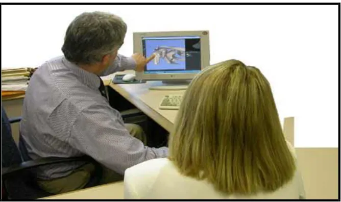
The physical world around us is in three-dimensional (3-D); yet traditional cameras and imaging sensors are only able to acquire and show two-dimensional (2-D) images that lack the depth information (Geng, 2011). The 2-D cross-sectional images produced from imaging techniques such as CT and MRI scanners are generally difficult to analyze. With this, the practice of surgical pathology involving the use of microscope to view tissue mounted on glass slides still persist significantly over many decades. In such usual cases of handling huge information embedded in each pixel of 2-D images, analyzing to deduce the position relationship between focus of infection and three dimensional geometry, estimating size and shape of focus of infection (Wu et al., 2010) usually require mental visualization of medical professionals based on their experience and expertise. This procedure is tedious, time-consuming and prone to error. Figure 1.1 and Figure 1.2 illustrate the conventional pathologist’s procedure of analyzing scanned images of patients and the visualization-assisted procedures respectively.
original volumetric data to renderable color and opacity values limit the application of volume rendering (Guo, Mao & Yuan, 2011).
Figure 1.1: Conventional pathologists’ slides viewing microscope (Jeong et al., 2010)
Figure 1.2: Clinical support with visualization
[image:23.612.161.495.359.557.2]such images (Yun & Xing, 2010). These medical scanners usually produce hundreds of 2-D slices requiring intense algorithm optimization. A computer-assisted brain diagnosis system that could effectively serve its purpose must be able to achieve not only fast generation of 3-D model of datasets but also the entire streams of datasets’ processing within an interactive speed. The promise of computer-based surgical planning is to provide better surgical results with fewer procedures, decreased time in the operating room, lower risk to the patients (increased precision of technique, decreased infection risk), and lower resulting cost (Kumar & Rakesh, 2011).
Most of the previously developed medical visualization systems have shortcomings in:
1. reconstructing 2-D sequence of human organ, soft tissue and lesions sectional images to 3-D model, (Geng, 2011; Wu et al., 2010).
2. detecting, mapping and isolating abnormalities / tumor for surgery and/or disease diagnosis procedure, (Kirmizibayarak et al., 2011; Gabor, et al., 2010; Guo et al., 2011).
3. handling mass data within a considerable interactive speed, extensive application interoperability and at a low resulting cost (Yun & Xing, 2010; Kumar & Rakesh, 2011).
1.4 Research Questions
This study aims to solve the following research questions:
1. How to reconstruct 2-D sequence of brain MRI into 3-D model?
2. How to detect, map and isolate brain abnormalities / tumor for surgery and/or disease diagnosis procedures?
3. How to handle mass volume of volumetric brain MRI datasets within a considerable interactive speed, extensive application interoperability and at a low resulting cost?
1.5 Research Objectives
The objectives for this research are as follows:
1. To propose new approaches for brain volume visualization by introducing a framework for reconstructing sequence of 2-D cross-sectional images to
3-D model,
a feature and edge detection scheme that can allocate transparency based on scalar values and assign transparency based on localized gradient magnitude for edge detection of region of interest in the data volume,
a technique with automatic local feature mapping scheme that can isolate abnormalities / tumor and reveal internal features of brain blood vessels, algorithms within the framework that are robust enough to handle mass
volumetric data within a considerable interactive speed, extensive application interoperability and at a lower resulting cost.
2. To design and implement a visualization system (SurLens) based on the proposed approaches.
1.6 Scope of the Research
This research focuses on the design of SurLens framework and the implementation of SurLens volume visualization system. The study is limited to reconstructing and locating
abnormalities / tumor in Magnetic Resonance (MR) Imagery of the brain in 3-D model. Focus is on obtaining quality 3-D images, sufficient enough to reveal detail internal information of datasets using the MRI datasets from the department of Surgery, University of North Carolina, Chapel Hill, United States. The study concentrates on Magnetic Resonance Angiography (MRA) datasets, however, Diffusion Tensor Imaging
(DTI), T1-Fast Low Angle Shot Magnetic Resonance (T1-FLASH) and T1-Magnetization Prepared Rapid Gradient Echo (T1-MPRAGE) would also be
considered. The development of the proposed visualization system would be within C# programming language environment, built on top of visualization toolkit (VTK) libraries and on parallel computing platform, Compute Unified Device Architecture (CUDA).
1.7 Organization of the thesis
To disseminate the findings of this research, concise investigation is presented into the field of visualization, human brain anatomy and its associated abnormalities.
Chapter 3 discusses the procedural research methodology, numerical computations and data structures used in the development of SurLens visualization system. The framework, schemes, algorithms, techniques and data collection for the development of SurLens visualization system are presented. Chapter 4 focuses on the designs and implementation of the proposed SurLens Visualization system for volumetric brain MRI datasets.
CHAPTER 2
VISUALIZATION OF VOLUMETRIC DATASETS
2.1 Introduction
Visualization is a phenomenon existing in our day-to-day life. Over a thousand years ago, visualization has been used in the data plots, maps and scientific drawings. As far back as 1137 A.D, visualization was used to draw the map of China and the very famous map of Napoleon’s invasion of Russia in 1812 (Owen, 1993). Visualization could be defined as a tool or method for interpreting image data, fed into a computer and for generating images from complex multi-dimensional data sets (McCormick, DeFanti & Brown, 1987). Informally, visualization engages the human vision and the processing power of human mind in the transformation of data or information into visual images referred to as pictures.
World Wide Web, directory or file structures on a computer or abstract data structures (InfoVis, 1995).
Visualization is also seen as a method of extracting meaningful information from complex dataset through the use of interactive graphics and imaging (Kaufman, Cohen & Yagel, 1993), hence, computer graphics and image processing (or imaging) are tools for visualization. Computer graphics is the creation of images using computer, which encompasses 2-D paint techniques, drawing or rendering techniques. The output of computer graphics is an image. With image processing, we can define techniques to transform (rotate, scale, shear), extract, analyze and enhance images. Visualization focuses on exploring, transforming, viewing data as image in order to gain understanding and insight into the data. Computer graphics is used as a tool to produce the output for visualization. However, this study specifically tread the path of volume visualization, which is typically identified with the rendering, modeling, manipulation and representation of datasets (Kaufman, 1991; Kaufman, 1996).
Volume visualization is an important diagnostic tool in modern medicine. With computer imaging techniques such as Computed Tomography (CT) and Magnetic Resonance Imaging (MRI), internal information of a living patient is captured. The information is captured in form of slice-planes or cross-sectional images of patient which could be compared to the conventional photographic X-ray. A slice consists of a series of number values representing the attenuation of X-rays (in case of CT) or the relaxation of nuclear spin magnetization (MRI) (Krestel, 1990). However, with applied and sophisticated mathematical techniques, the slice-planes could be reconstructed and gathered into a volume of data.
This chapter reviews visualization of volumetric datasets and presents earlier frameworks from which medical volume visualization can be facilitated. After outlining broad collection of volumetric data acquisition methodologies, varying volume rendering techniques are described. The chapter extrapolates image reconstruction approaches, direct volume visualization techniques; possible optimization procedures specifically parallel processing approaches and their outstanding issues, which crystalize the research direction for this study. The weaknesses and strengths of each of the previous techniques are discussed. The strengths and weaknesses of ten (10) recently proposed volume visualization frameworks in entirety, including their proposed schemes, algorithms and techniques, are presented and compared in justification of the proposed framework, schemes, algorithms and technique in this study.
2.2 Volume Visualization
Volume visualization is a sub-field of scientific visualization that extracts meaningful information from volumetric data using interactive graphics and imaging, and it is concerned with volume data representation, modeling, manipulation, and rendering (Suter et al., 2011). Volume visualization is an important tool for visualizing and analyzing data sets with its extensive application into such areas as biomedicine, computational fluid, finite element models, computational chemistry and geophysics. Magnetic Resonance (MR) Imagery and Computed Tomography (CT) are both imaging techniques benefiting optimally from volume visualization. Such numerical simulations and sampling devices create images of the human body for clinical diagnosis while volume visualization presents such datasets for viewing and clinical analyzing of the anatomical structures. Over recent years, volume visualization is continually evolving as visualization approaches, especially with the advent of faster processing devices. One of the challenges depriving the usage of volume visualization is the memory system to support volume processing (Suter et al., 2011; Ma, Murphy & O’Mathura, 2012).
its other sides, will become a line. Hence, a 2-D structure has corners or vertices and sides in two planes and cannot provide detail information embedded in image data. However, the 2-D representation can be re-represented in three-dimension (3-D), using mathematical models which has X and Y planes (just as 2-D image) but a Z-axis inclusive, this gives the image more features such as rotation. This third axis added faces to the 3-D structures, making the data available for real world simulation of the imaged object.
Since, there is a one-to-one correspondence between the pixel value in the image scan and a specific tissue of a patient, the numbers could be assigned a specific gray scale value. Displaying the data on the computer screen at this stage will emerge the structures in the patient’s data. The emerged structures are as a result of the interaction of the human visual system with data spatial organization and the chosen gray-scale values. With this approach, its being possible to translate what computer represents as series of numbers into the corresponding cross-section of human body; the skin, the bone and the tissue. A more useful result could be made available for diagnosis by extending the 2-D into 3-D technique. In this case, the image slices are gathered as a volume of data. With 3-D technique, we can reveal the entire anatomical structure of a living patient without the intervention of surgery.
With the inability of the medical image scanners to present human anatomical structures in 3-D format, reconstruction procedure is the alternative. Reconstruction is a reverse engineering technique of 2-D MR imagery to 3-D. This is achieved in the medical diagnosis and disease management using the combination of computer graphics and image processing tools, the resulting 3-D data could serve as information for opinion making and intervention planning on a living patient without any prior
mandatory surgical operation.
2.3 Volumetric Image Datasets
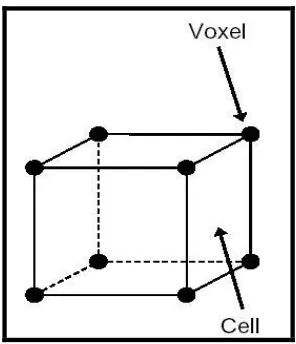
with d representing the data property at a location determined by x,y,z. To describe value at any d continuous location, zero-order (the Nearest Neighbor), first-order (trilinear also called piecewise function) and higher-order interpolation are possible options. The
region of constant value that surrounds each sample in zero-order interpolation is known as a volume cell (commonly interchangeably referred to as voxel (volume element) or grid location or sample points) with each voxel being a rectangular cuboid
having six faces, twelve edges and eight corners (Kaufman, 1996). Dataset is a collection of volume elements. However, there is variation in the spatial and intensity resolution of images produce by different medical imaging devices. This section presents some of the commonly used tools for volume data acquisition.
It is important to discuss the topology or geometry in which volumetric data must be. Data samples may exist as scalar data, holding such values as temperature, pressure and density, or exist as vector (e.g. velocity) or tensor (e.g. Finite Element Methods (FEM) modeling). Typically, a volume dataset V is a set of element (Winter, 2002) defined as:
{
V
i(
x
,
y
,
z
)
i
1
,
2
,...,
n
}
)
,
,
(
x
y
z
is a point in 3-D space, 3)
,
,
(
x
y
z
i
could be scalar, vector or tensor, which is defined as follows: a scalar function f : 3 ;
an n-dimensional vector function, fn : 3 n, or a k-ranked tensor function, :
k n
f 3 ,
k n
Scalar and vector functions are representation of special cases of tensor functions with
Figure 2.1: Volumetric Data in Cartesian Grid
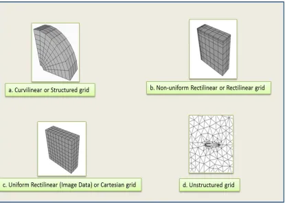
Speray & Kennon (1990) categorized volume dataset V into structured and unstructured based on the topology of the dataset. In line with such categorization, the
Figure 2.2: Data Structure Grids
2.4 Medical Imaging Modalities
Volume visualization became feasible with the revolution in image acquisition for extensive medical diagnosis and pre-treatment planning. The medical science that uses electromagnetic radiation, ultrasonography or radioactivity for evaluation of body tissues in case of injury or disease is referred to as diagnoses medical imaging. However, electromagnetic radiation can either be ionizing or non-ionizing. This section gives a brief overview and concepts of some of medical imaging modalities.
principle for using X-ray involves passing of beam of X-rays, produced by an X-ray tube to selected parts of the body. There was an attempt to reconstruct images from projections as at 1940, this was even planned before the advent of modern computer technology. Gabriel Frank achieved this with the plan of describing the basic idea of modern tomography including such concepts as sonograms and optical back projection (Hsieh, 2002). About 16 years later, Allah M. Cormack furthered the research objectives with some experimental works based on reconstructive tomography.
In 1967, the first CT scanner was developed by Godfrey N. Hounsfield in England at the Central Research Laboratory of EMI, Ltd (Hounsfield, 1973). Hounsfield investigation on pattern recognition techniques shows that if X-ray is passed through a body from different directions, this would result in its’ internal body reconstruction. In his trials in 1969, test objects were scanned with isotope source that required a scan time of 9 days per image (Kalender, 2006).
Research usage of any of the image modalities depends on the intended image area to extract. Some could successfully extract certain information called “Morphological Information” while others are very useful in extracting “physiological or functional information”. X-ray, CT and MRI are typical examples of former while
PET and SPECT are examples of the later. However, such specific features and
functionalities justify their usage in medical community. Section 2.4.3 explains specific clinical relevancies of these image modalities.
2.4.1 Computed Tomography
Computed tomography (CT) is a widely adopted imaging modality with many clinical applications from diagnosis to procedure planning (Merck, 2009). Computed Tomography is a technique of X-ray photography in which a single plane of a patient is scanned from various angles in order to provide a cross-sectional image of the internal structure of that plane (Hsieh, 2002). Conventional radiography uses the relative
distribution of X-ray intensities for its measurement. It involves sending of uniform intensity X-ray through a patient from an X-ray source of intensity Io and corresponding exiting of the X-ray with intensity I (x, y) from the other side, which then interact with a radiography film sheet. The different paths through the material will alternate the X-rays by varying amounts, based only on the mass attenuation coefficient (µ), since the distance (d) is the same on all point of the radiography film (Shabaneh et al., 2004). CT
uses attenuation as the judgments of its measurements as the X-ray is scanned through the patients.
Figure 2.3: An example of a CT slice, a head scan (Lundström, 2007)
The patient is scanned using an X-ray source from one side of the plane and the detector placed on the opposite side is used to measure the attenuated X-ray, which is recorded by computer. After the first scan through the plane, the X-ray source and the detector rotate with a particular predefined amount for another translational scan. Hence, an X-ray technique involves passing electromagnetic radiation through the body. This is usually presented as CT Number, expressed in “Hounsfield Units” or “HU” named after Godfrey Hounsfield. A positive CT indicates a tissue is more attenuating than water while a negative CT denotes a tissue with lower density than water.
2.4.2 Magnetic Resonance Imaging
different from that of Computed Tomography as it uses energy sources as its imaging procedure rather than ionizing radiation technique of X-ray. In the early years of existence of MRI, it was referred to as Nuclear Magnetic Resonance Imaging (NMRI) since it was developed from knowledge gained in the study of nuclear magnetic resonance (Amruta, Gole & Karunakar, 2010). The term NMRI is sometimes still in use when discussing non-medical devices of the same NMRI principle. However, in medical imaging, magnetic resonance tomography (MRT) may sometimes be interchangeably used for MRI. The procedure requires the usage of a strong magnetic field for spin alignment of hydrogen nuclei (photons) in the body.
The spin synchronizes as the radio-frequency (RF) pulse matches the nuclear resonance frequency of the photons. As the pulse is removed, different relaxation times are measured, that is, the times for the spins to go out-of-sync (Lundström, 2007). The density and chemical surroundings of the hydrogen atoms determine the measured value. Whilst some vectors will form alignment towards the direction of the main magnetic field, a slight majority will align themselves in the slightly lower energy state associated with the direction of the main magnetic field (Geoffrey et al., 2008). MRI creates its images as a result of the difference between two populations of vectors leading to the equilibrium net magnetic vectors. We could therefore say that, with MRI, a body is prepared for radio signal transmission on the FM bandwidth. The relative distribution of the vectors aligned within or against the main magnetic field is described by Boltzmann distribution as in equation (2).
The value of k is the Boltzmann constant, T is the temperature measured in kelvin, h is the Planck constants, γ is the gyromagnetic ratio of the nucleus in rad/T/s and B is
the strength of the magnetic field in tesla, ∏ is a constant approximately equal to 3.14159. The number of spins in the lower energy level and the number of spins in the upper energy level are denoted by n↑ and n↓ respectively.
Figure 2.4: An example of an MRI slice, brain’s Scan
2.4.3 Clinical Applications / Relevancies
MRI is the only chemically sensitive in-vivo imaging technique with high-resolution soft tissue contrast that allows physicians to peer deep inside the human body, producing clinically relevant images of soft tissue lesions and functional parameters of the body organs, without the use of invasive procedures or ionizing radiation such as X-rays (Cosmus & Parizh, 2011). However, with the knowledge gained in the course of this study, some of the clinical applications of CT and MRI, as being proven by researchers, solemnly depend on the required medical examination on the patient and in certain cases, the image modalities are seen to be complementary to each other in the diagnosis procedures.
2.5 Dataset Pre-Processing Techniques
Pre-processing stage in volume visualization is to enhance the visual appearances of the images and the manipulation of the datasets’ structures, to convert them from their acquired representation to spatial representation required and appropriate for visualization. However, a lot of caution needs to be exercised with image enhancements’ procedures as poorly embarked approach may introduce image artefacts or even lead to loss of information in the datasets.
Segmentation, a key step and a large research area in visualization, is usually performed at the pre-processing step of volume visualization. As a matter of fact, different organs or tissues of an acquired volumetric data might have the same density or intensity hence segmentation stage and not only classification becomes essential. The fundamental principle guiding volume visualization is based on the fact that empowering the user to see a certain structure, using only classification is not always possible (Meißner et al., 2000). Though acquisition methods usually demand different level or extent of required segmentation but most methods require semi-automatic approach which invariably increases the overall processing time of datasets in volume visualization. Studies have shown that segmentation of brain MR is a compulsory, difficult and time consuming stage for volume visualization because of variable imaging parameters, overlapping intensities, noise, partial voluming, gradients, motion, echoes, blurred edges, normal anatomical variations and susceptibility artefacts (Lladó et al., 2012; Sha & Sutton, 2001).
This section reviews previous datasets pre-processing techniques and highlights the significant contribution of SurLens Dataset Pre-processing approach.
2.5.1 Filtering, Enhancement, Detection & Extraction
2012), wavelet-based thresholding (Agrawal & Sahu, 2012), anisotropic non-linear diffusion filtering (Zhang & Ma, 2010; Perona & Malik, 1990), Markov Random Field (MRF) models (An & An, 1984), wavelet models (Nowak, 1990), non-local means modes (NL-means) (Buades, Coll & Morel, 2005), and analytical correction schemes (Sijbers, 1998). Despite the fact that there are quite a substantial number of state-of-the-art methods for de-noising, accurate removal of noise from MRI is still a challenge; as all these methods are almost the same in terms of computation cost, de-noising, quality of de-noising and boundary preserving, which has retained MRI de-noising as an open issue that needs better improved methods (Bandhyopadhyay & Paul, 2012). Hence, de-noising methods at this current state of research are not reliable enough to fully support pre-processing stage of volume visualization. The main challenge in de-noising MRI is to preserve the edges and the details, at the same time to reduce noise in uniform regions (Diaz et al., 2011).
Edge detection or extraction is an important step in MRI data pre-processing. There are three steps in edge detection process (Senthilkumarn & Rajesh, 2008), the image filtering, the image enhancement, and the image detection. Image filtering is required in pre-processing because the target MRI images might have been corrupted through a number of circumstances like impulse noise, Gaussian noise, being common situations. More filtering procedures to reduce noise may results in loss of the strength of the edges (Senthilkumarn & Rajesh, 2009). Image enhancement emphasizes pixels where there is a significance change in local intensity values and is usually performed by computing gradient magnitude (Wen, Zhang & Jiang, 2008) while image detection usually based on threshoding criterion (Paulinas & Usinskas, 2007).
contributing approach must be considered during the pre-processing stage of a volume visualization framework in order to improve accuracy and noise sensitivity interference. As one of our contributions to this field, we have therefore designed and implemented a new algorithm for image filtering, enhancements, detection and extraction, actualized at the graphic execution phase of our framework, which is the main entry point of datasets into volume visualization. This is an improved and better approach tackling accuracies of image filtering, enhancements, detection and extraction by enabling the datasets to be processed at the main entry point of volume visualization in order to avoid any unwanted noise sensitivity. We do not observe any shortcoming of this design hence it is noted as an improvement over all the previously pre-processing approaches.
2.5.2 Volume Segmentation
Brain MRI segmentation has been attracting attention for a while considering its significance in the medical image analysis and diagnosis. As each of the points in the image scan corresponds to a particular point in the human body structure, during segmentation process, each point in the scanned image and its correspondence to the tissue or organ is identified. A number of segmentation algorithms have been proposed in the past. Clustering-based (Kannan & Pandiyarajan, 2009), region-growing (Welinski & Fabijanska, 2011; Deng et al., 2010), active contour-based (Tanoori et al., 2011), watershed-based (Freitas et al., 2011) and morphological-based segmentation (Li et al., 2011) have been previously applied to brain MRI volume segmentation. Sethian (1999), Ben-Zadok, Riklin-Raviv & Kiryati (2009) and Cremers et al., (2007) have made appreciable contribution in the boundary-based segmentation procedures.
unsupervised strategy performs brain MRI segmentation with no prior knowledge or information. The supervised methods are listed to include Bayes classifiers with labeled maximum likelihood estimators, the k-nearest neighbour rule (kNN) and artificial neural networks (ANN) while the unsupervised methods include Bayes classifiers with unlabelled maximum likelihood estimators or the fuzzy C-means (FCM) algorithms. Though segmentation is usually performed at the pre-processing stage of volume visualization, being a key and a large research area, some studies separated the usual pre-processing stages distinctly from segmentation. Clarke et al. (1995) reviewed both pre-processing and segmentation methods of soft brain tissue. In the same vein, Styner et al. (2008) reviewed semi-automated and automated multiple sclerosis (MS) lesion segmentation approaches, analyzing MS lesions, pre-processing steps and segmentation approaches. More recently, Lladó et al. (2012) presented a review of brain MRI with the goal of helping diagnosis and follow-up of multiple sclerosis lesions in brain MRI. In order to enhance the visual appearance of the brain MRI images, any possible artefacts will need to be removed. Removal of the contained artefacts could be done at this stage, done partly or delayed until the final entry point of the dataset into volume visualization phase, this depends on the design of the volume visualization framework. Whichever of the approach being adopted in the framework design, there must be adequate provision set aside in case of unexpected introduction of certain level of artefacts during the pre-processing phase.
Skull stripping is another important pre-processing step since fat, skull, skin and other non-brain tissues may cause mis-classifications in some approaches due to the intensity similarities with brain structures (Detta & Narayana, 2011). Some of the components of the brain require a particular MRI technique for their diagnosis, hence, without thorough skull stripping it might be difficult to have the intended structures’ of study visible with volume visualization algorithms.
REFERENCES
Agrawal, S. & Sahu, R. (2012).Wavelet Based MRI Image Denoising Using Thresholding Techniques. International Journal of Science, Engineering and Technology Research (IJSETR). Vol. 1, Issue 3, September.
Ahrens, J., Geveci, B., & Law, C. (2005). The Visualization Handbook, ParaView: An End-User Tool for Large Data Visualization. Burlington, MA: Elsevier, 717.
Alim, U.R. & Möller, T. (2009). A Fast Fourier Transform with Rectangular Output on the BCC and FCC Lattices.Proc. Eighth Int’l Conf. Sampling Theory and Applications (SampTA).
Aliroteh, M. & McInerney, T. (2007). SketchSurfaces: Sketch Line Initialized Deformable Surfaces for Efficient and Controllable Interactive 3D Medical Image Segmentation, Third International Symposium on Visual Computing (ISVC), LNCS 4841, Lack Tahoe, Nevada/California, November 26-28, pp. 542-553.
Amruta, A., Gole, A. & Karunakar, Y. (2010). A Systematic Algorithm for 3-D Reconstruction of MRI based Brain Tumorusing Morphological Operations and Bicubic Interpolation. 2nd International Conference on Computer Technology and Development (KCTD).
An, S. & An, D. (1984). Stochastic Relaxation, Gibbs Distributions, and the
Bayesian Restoration of Images. IEEE Trans Pattern Anal Mach Intell6: 721–741.
Baek, S.Y., Sheafor, D.H., Keogan, M.T., DeLong, D.M. & Nelson, R.C. (2001). Two-dimensional multiplanar and three-dimensional volume-rendered vascular CT in pancreatic carcinoma: interobserveragreement and comparison with standard helical techniques. Am J Roentgenol 176(6):1467–1473.
Bandhyopadhyay, S.K. & Paul, T.U. (2012). Segmentation of Brain MRI Image A Review. International Journal of Advanced Research in Computer Science and Software Engineering. Volume 2, Issue 3, March 2012 ISSN: 2277 128X.
Bentoumi, H., Gautron, P. & Bouatouch, K. (2010). GPU-Based Volume Rendering for Medical Imagery. International Journal of Electrical, Computer, and Systems Engineering 4:1.
Ben-Zadok, N., Riklin-Raviv, T. & Kiryati, N. (2009). Interactive level set segmentation for image-guided therapy. In IEEE Int. Symp. On Biomedical Imaging, pages 1079–1082.
Benzinga News. November 29, 2010. Kitware Offers Free Global Access to VolView at RSNA.
Bezdek, J.C., Hall, L.O. & Clarke, L.P. (1993). Review of MR Image Segmentation Techniques using Pattern Recognition, Med. Phys. 20 (4) 1033–1048. Birk, M., Guth, A., Zapf, M., Balzer, M., Ruiter, N., Hübner, M. & Becker, J. (2011).
Acceleration of Image Reconstruction in 3D Ultrasound Computer Tomography: An Evaluation of CPU, GPU AND FPGA Computing. IEEE Conference on Design and Architectures for Signal and Image Processing (DASIP). On page(s): 1 – 8, E-ISBN : 978-1-4577-0619-6, Print ISBN: 978-1- 4577-0620-2.
Bredel, M. (2009). Gene Connections Key to Brain Tumor. Journal of the American Medical Association.The U.S. National Cancer Institute, Cancer Newsletter. July, 20.
Topology-Based Data Segmentation. IEEE Transactions on Visualization And Computer Graphics, Vol. 17, No. 9, pp. 1307- 1324.
Buades, A., Coll, B. & Morel, J. (2005). A Non-Local Algorithm for Image Denoising. IEEE Computer Society Conference on Computer Vision and Pattern Recognition, pp 60–65.
Bullitt, E., Zeng, D., Mortamet, B., Ghosh, A., Aylward, S.R., Lin, W., Marks, B.L. & Smith, K. (2010). The Effects of Healthy Aging on Intracerebral Blood Vessels Visualized by Magnetic Resonance Angiography: Neurobiol Aging 31(2): 290–300.
Busking, S. Vilanova, A. & Wijk, J.V. (2007). Particle-Based Non- Photorealistic Volume Visualization,” Visual Computer, vol. 24, No. 5, pp. 335-346, May 2007.
Cao, Y., Wu, G. & Wang, H. (2011). A Smart Compression Scheme for GPU-Accelerated Volume Rendering of Time-Varying Data. IEEE International Conference on Virtual Reality and Visualization, Page(s): 205 – 210.
Carlos, D.C. & Ma, kwan-Liu (2009). The occlusion spectrum for volume classification and visualization, IEEE Transactions on Visualization and Computer Graphics, Vol. 15, No. 6.
Chen, C. & Yang, J. (2011). Essence of Two-dimensional Principal Component Analysis and Its Generalization: Multi-dimensional PCA. Second International Conference on Innovations in Bio-inspired Computing and Applications.IEEE Computer Society.
Chen, M., Kaufman, A. & Yagel, R. (2000). Volume Graphics, Springer (Eds.). London.
Chen, Ming-Da., Hsieh, Tung-Ju. & Chang, Yang-Lang. (2011). Volume Data Numerical Integration and Differentiation Using CUDA. IEEE 17th International Conference on Parallel and Distributed Systems.
Cheung, M.R. & Krishnan, K. (2012). Using Manual Prostate Contours to Enhance Deformable Registration of Endorectal MRI. Computer Methods
Chiueh, T.-C., Yang, C.-K., He, T., Pfister, H. & Kaufman, A.E. (1997). Integrated Volume Compression and Visualization. In Proc. IEEE Visualization, Pages 329–336. Computer Society Press.
Chiw, C., Kindlmann, G., Reppy, J., Samuels, L. & Seltzer, N. (2012). Diderot: A Parallel DSL for Image Analysis and Visualization. Proceedings of the 33rd ACM SIGPLAN conference on Programming Language Design and Implementation. ACM New York, NY, USA, pp 111-120.
Chu, H., Chen, L. & Yong, J. (2010). Feature variation curve guided transfer function design for 3D medical image visualization, 3rd International Conference on Biomedical Engineering and Informatics.
Clarke,L.P., Velthuizen, R.P., Camacho, M.A., Heine, J.J., Vaidyanathan, M., Hall, L.O., Thatcher, R.W. &Silbiger, M.L. (1995). MRI Segmentation: Methods and Applications, Magn. Reson.Imag. 13 (3)
343–368.
Cosmus, C. C & Parizh, M. (2011). Advances in Whole-body MRI Magnets. IEEE transactions on applied semiconductivity , Vol. 21, No. 3.
Courchesne, E., Chisum, H.J., Townsend J, Cowles, A., Covington, J., Egaas, B., Harwood, M., Hinds, S. & Gary, A. (2000). Normal Brain Development and Aging: Quantitative Analysis at in vivo MR Imaging in Healthy
Volunteers.Journal of Radiology. Press GA. 216:672–682. [PubMed: 10966694].
Cox, G., Maximo, A., Bentes, C. & Farias, R. (2009). Irregular grid Raycasting
implementation on the cell broadband engine, 21st International Symposium on Computer Architecture and High Performance
Computing.
Creasey, H. (2003). Rapoport SI. The aging human brain. Annals of Neurology. 17:2–10. [PubMed:3885841].
Csébfalvi, B. & Domonkos, B. (2009). Frequency-Domain Upsampling on a Body-Centered Cubic Lattice for Efficient and High-Quality Volume Rendering. Conference on Vision Modeling and Visualization – VMV, pp. 225-232. Csébfalvi, B. & Szirmay-Kalos, L. (2003).Monte Carlo Volume Rendering. Proc. of
IEEE Visualization, pp.449- 456, 2003.
Da Silva, L.S., & Scharcanski, J. (2005). A lossless Compression Approach for Mammographic Digital Images Based on the Delaunay Triangulation. IEEE International Conference on Image Processing, ICIP. pp.11 - 758-61.
Damadian, R., Goldsmith, M. & Minkoff, L. (1977). NMR in cancer: XVI. Fonar image of the live human body”, Physiological Chemistry and Physics, Vol. 9, pp. 97-100.
Datta, S. & Narayana, P.A. (2011). Automated Brain Extraction from T2- Weighted Magnetic Resonance Images, J. Magn.Reson. 33 (4) 822– 829.
Deng, W., Xiao, W., Deng, E. & Liu, J. (2010). MRI Brain Tumor Segmentation With Region Growing Method Based On The Gradients andVariances Along And Inside Of The Boundary Curve. 3rd International Conference on Biomedical Engineering and Informatics (BMEI).
Diaz, I., Boulanger, P., Greiner, R. & Murtha, A. (2011). A Critical Review of the Effect of De-noising Algorithms on MRI Brain Tumor Segmentation. 33rd Annual International Conference of the IEEE EMBS, Boston, Massachusetts, USA.
Dorgham, O.M., Laycock, S.D. & Fisher, M.H. (2012). GPU Accelerated Generation of Digitally Reconstructed Radiographs for 2-D/3-D Image
Registration. IEEE Transactions on Biomedical Engineering, Vol. 59, No. 9. Pp. 2594 – 2603.
Drebin, R., Carpenter, L., Hanrahan, P. (1988). Volume rendering, Proceedings SIGGRAPH88, pp 65–74.
Ferre, M., Cobos, S., Aracil, R. & Sánchez Urán, M.A. (2007). 3D Image Visualization and Its Performance in Teleoperation, HCI. International Conference, Peking, China. Virtual Reality, Vol.14, LNCS 4563, R. Shumaker (Hrg.); Springer, Volume 14, LNCS 4563, pp 669-707.
Freitas, P., Rittner, L., Appenzeller, S. & Lotufo, R. (2011). Watershed-based Segmentation of the Midsagittal Section of the Corpus Callosum in Diffusion MRI. 24th Conference on Graphics, Patterns and Images 2011 24th SIBGRAPI Conference on Graphics, Patterns and Images. Pg 274-280.
Frigo, M. & Johnson, S. (2005). The Design and Implementation of FFTW3. Proc. of the IEEE, 93(2): 216-231.
Gabor J. Tornai, G.J. & Cserey, G. (2010). 2D and 3D Level-Set Algorithms on CPU. 12th International Workshop on Cellular Nanoscale Network and their Applicatins (CNNA).
Geng, J. (2011). Structured-light 3D surface imaging: a tutorial. Advances in Optics and Photonics 3, 128-160.
Geoffrey S.P., Elizabeth, Charles-Edwards & Christopher, P. (2008). Applications of Computed Tomography, Magnetic Resonance Imaging and Magnetic Resonance Spectroscopy for Planning External Beam Radiotherapy, Current Medical Imaging Reviews, 4, 236-249.
Ghorpade, J., Parande, J., Kulkarni, M. & Bawaskar, A. (2012). Gpgpu Processing in Cuda Architecture. Advanced Computing: An International Journal (ACIJ ), Vol.3, No.1.
Gong, F. & Zhao, X. (2010). Three-Dimensional Reconstruction of Medical Image Based on Improved Marching Cubes Algorithm. International Conference on Machine Vision and Human-machine Interface.
GPU Computing and the CUDA architecture (2009). NVIDIA CUDA Architecture Introduction & Overview, Version 1.1.
Algorithm. Computerized Medical Imaging and Graphics. Computerized Medical Imaging and Graphics 36 560– 571.
Guo, H., Mao, N. & Yuan, X. (2011). WYSIWYG (What You See is What You Get) Volume Visualization. IEEE Transactions on Visualization and Computer Graphics, Vol. 17, NO. 12, on page(s): 2106 – 2114, ISSN : 1077-2626.
Guo, H., Xiao, H. & Yuan, X. (2012). Scalable Multivariate Volume Visualization and Analysis Based on Dimension Projection and Parallel
Coordinates. IEEE Transactions on Visualization and Computer Graphics, Vol. 18, No. 9, pp 119-120.
Guo, H., Xiao, H. & Yuan, X. (2011). Multi-Dimensional Transfer Function Design Based on Flexible Dimension Projection Embedded in Parallel Coordinates. Proc. IEEE Pacific Visualization Symp., pp. 19-26.
Gupta, D., Anand, R.S., & Tyagi, B. (2012). Enhancement of Medical Ultrasound Images using Non-Linear Filtering Based on Rational-Dilation Wavelet Transform. Proceedings of the World Congress on Engineering and Computer Science (WCECS).Vol. I October 24-26. San Francisco, USA Hadwiger, M., Kniss, J., Rezk-Salama, C., Weiskopf, D. & Engel, K. (2006).
Real-time volume graphics, A K Peters Publications.
He, X. (2009). Reconstruction of 3d microstructure of the rock sample Basing on the CT images. Proceedings of the International Conference on Wavelet Analysis and Pattern Recognition, Baoding, 12-15 July.
Hege, H.C., Höllerer, T. & Stalling, D. (1996). Volume Rendering - Mathematicals Models and Algorithmic Aspects. W. Nagel (Hrsg.) PartielleDifferentialgleichungen, Numerik und Anwendungen. Konferenzen des ForschungszentrumsJülich GmbH, S. 227-255.
Hernell, F., Ljung, F. & Ynnerman, A. (2010). Local ambient occlusion in direct volume rendering, IEEE Transactions on Visualization and Computer Graphics, Vol. 16, No. 4.
Hong, L. & Shuhuil, M. (2010). High Precision Hybrid Technique of Surface and Volume Rendering. Second International Conference on Computational Intelligence and Natural Computing (CINC).
Hossain, Z., Alim, U.R. & Möller, T. (2011). Toward High-Quality Gradient Estimation on Regular Lattices. IEEE Transactions on Visualization and Computer Graphics, Vol. 17, No. 4, pp. 426 – 439.
Hounsfield G.N. (1973). Computerized transverse axial scanning tomography, Description of system Br. J. Radiol., 46 1016.
Hsieh, J. (2002). Computed Tomography Principles, Design, Artifacts, and recent Advances, Spie Press.
Hu, S. & Hou, W. (2011). Denosing 3D Ultrasound images by Non-local Means Accelerated by GPU. IEEE International Conference on Intelligent Computation and Bio-Medical Instrumentation, pp. 43-45.
Jeong, Won-Ki., Schneider, J., Turney, S.G., Faulkner-Jones, B.E., Meyer, D., Westermann, R., Reid, R.C., Lichtman, J. & Pfister, H. (2010). Interactive Histology of Large-Scale Biomedical Image Stacks. IEEE Transactions on Visualization and Computer Graphics, Vol. 16, no. 6, November/December.
Jinzhu, Y., Fangfang, H., Chaolu, F., Dazhe, Z. & Yanfei, W. (2011). An Accelerative Method for Multimodality Medical Image Registration Based
on CUDA. 4th International Congress on Image and Signal Processing (CISP), pp. 1817 – 1821.
Joemai, R.M.S., Geleijns, J., Veldkamp, W.J.H., De Roos, A. & Kroft, L.J.M. (2008). Automated cardiac phase selection with 64-MDCT coronary angiography, AJR Am J Roentgenol 191:1690–1697.
Kainz, B., Portugaller, R.H, Seider, D., Moche, M., Stiegler , P. & Schmalstieg, D. (2011). Volume visualization in the clinical practice. Augmented Environments for Computer Assisted Interventions (AE-CAI'11).
Kalender, W.A. (2006). Review: X-ray Computed Tomography, Institute of Physics Publishing Phys. Med. Biol. 51, R29–R43.
Kannan, S.R. & Pandiyarajan, R. (2009). Effective fuzzy c-mean Clustering technique for segmentation of T1-T2 brain MRI. IEEE International Conference on Advances in Recent Technologies in Communication and Computing. Pg. 537-539.
Kasiri, K., Dehghani, M.J., Kazemi, K., Helfroush, M.S. & Kafshgari, S. (2010). Comparison Evaluation of Three Brain MRI Segmentation Methods
in Software Tools. IEEE Proceedings of the 17th Iranian Conference of Biomedical Engineering (ICBME).
Kasthuri, N. & Lichtman, J.W. (2010). Neurocartography, Neuropsychopharmacology, 35, 342–343; doi:10.1038/npp.2009.138. Kaufman, A. (1991). Volume Visualization (Tutorial). IEEE Computer Society
Press, Los Alamitos, California.
Kaufman, A. & Mueller, K. (2005). Overview of Volume Rendering, The Visualization Handbook, eds. C. Johnson and C. Hansen, Academic Press. Kaufman, A.E. (1996). Volume Visualization. ACM Computing Survey, 28(1):
165-167.
Kaufman, A.E. (2000). Volume visualization: Principles and advances. International Spring School on Visualization, Bonn.
Kim, J. & Jaja, J. (2009). Streaming Model Based Volume Ray Casting
Implementation for Cell Broadband Engine, Scientific Programming, Vol. 17, no. 1-2, pp. 173-184.
Kirk, D. & Hwu, W.-M. (2010). Programming Massively Parallel Processors: A Hands-on Approach. Morgan Kaufmann, 2010.