Forecasting Electricity Consumption Using SARIMA Method in IBM SPSS Software

(1)

Universal Journal of Electrical and Electronic Engineering 6(5B): 103-114, 2019 http://www.hrpub.org DOI: 10.13189/ujeee.2019.061614

Forecasting Electricity Consumption Using SARIMA

Method in IBM SPSS Software

Sze En Sim1, Kim Gaik Tay1,*, Audrey Huong1, Wei King Tiong2

1

Faculty of Electrical and Electronics Engineering, Universiti Tun Hussein Onn Malaysia, Malaysia

2

Faculty of Computer Science and Information Technology, Universiti Malaysia Sarawak, Malaysia

Received July 26, 2019; Revised September 24, 2019; Accepted December 22, 2019

Abstract

Forecasting is a prediction of future values based on historical data. It can be conducted using various methods such as statistical methods or machine learning techniques. Electricity is a necessity of modern life. Hence, accurate forecasting of electricity demand is important. Overestimation will cause a waste of energy but underestimation leads to higher operation costs. Univesity Tun Hussein Onn Malaysia (UTHM) is a developing Malaysian technical university, therefore there is a need to forecast UTHM electricity consumption for future decisions on generating electric power, load switching, and infrastructure development. The monthly UTHM electricity consumption data exhibits seasonality-periodic fluctuations. Thus, the seasonal Autoregressive Integrated Moving Average (SARIMA) method was applied in IBM SPSS software to predict UTHM electricity consumption for 2019 via Box-Jenkins method and Expert Modeler. There were a total of 120 observations taken from January year 2009 to December year 2018 to build the models. The best model from both methods is SARIMA(0, 1, 1)(0, 1, 1)12. It was found that the result through the Box-Jenkins method is approximately the same with the result generated through Expert Modeler in SPSS with MAPE of 8.4%.

Keywords

SARIMA, SPSS, Box-Jenkin Method, Expert Modeler, UTHM, Electricity Consumption

1. Introduction

Electricity is the most adaptable type of vitality and comprises one of the imperative infra-auxiliary contributions to financial improvement. Overestimation or underestimation of the electricity consumption would lead to superfluous idle capacity which means wasted financial

resources or causes higher operation costs for energy supplier and would cause potential energy outages. Therefore, modelling electricity consumption with good accuracy becomes vital to avoid costly mistakes and another unneeded effect. Forecasting is mean to predict the future via a set of statistical tools and techniques that are supported by human judgement and intuition. Forecasting is the use of a set of historical data to do an analysis and finally predict future data from the trend [1].

Various techniques have been applied in electricity consumption forecasting including holt-winters and seasonal regression [2], time series models [3], first-order fuzzy time series [4], multiple linear regression [5-6], autoregressive integrated moving average (ARIMA) [7], seasonal ARIMA (SARIMA) [8], artificial neural network (ANN) [6, 8-13], Least-square SVM (LSSVM) [13], support vector regression [9], ANFIS[14-15] and ARIMA-ANFIS [16].

UTHM is a developing Malaysian technical university, hence, there is a need to forecast UTHM electricity consumption for future decisions on generating electric power, load switching, and infrastructure development. Its monthly electricity consumption data from January year 2009 to December year 2018 was collected. The data exhibits seasonality-periodic fluctuations, therefore SARIMA was chosen to forecast the year 2019 consumption. SARIMA not only successfully forecasted electricity consumption but also dengue occurrence [17] and foreign tourism at the airport [18]. The best model of SARIMA following Box-Jenkins [19] methodology will be compared with Expert Modeler in IBM SPSS software.

2. SARIMA

(2)

φ φ φ

θ θ θ ε

− − − − − Φ − Φ − − Φ

− − =

+ + + + + Θ + Θ + + Θ

 

2 2

1 2 1 2

2 2

1 2 1 2

(1 )(1 )

(1 ) (1 )

(1 )(1 )

p P

d D

t

q Q

q Q t

B B B B B B

B B y

B B B B B B

or

φ( ) ( )(1Φ S − ) (1d − S D) =θ( ) ( )Θ S ε p B p B B B yt q B Q B t

where φ θ, are parameters of autoregressive (AR) and moving average (MA), while Φ Θ, are parameters of seasonal autoregressive (SAR) and seasonal moving average (SMA) respectively. Meanwhile, p, d, q are the orders of autoregressive, AR(p), difference and moving average MA(q), whereas P, D, Q are the orders of seasonal autoregressive SAR(P), seasonal difference and seasonal moving average SMA(Q) respectively. S is the seasonal length, y_t is predicted variable and εtis a random error at

time t.

3. Materials and Methods

In this study, two approaches to implement SARIMA which are Box-Jenkins methodology and Expert Modeler in IBM SPSS will be discussed. The monthly UTHM electricity consumption from January year 2009 to December year 2018 was collected from Development and Maintenance Office, UTHM.

3.1. Box-Jenkins Methodology

Box-Jenkins methodology involves 5 steps as follows:

 the data characteristics,

 model identification,

 parameters estimation,

 diagnostics for getting the best model,

 forecasting

3.2. Expert Modeler

The expert modeler is a black box tool provided in SPSS to implement SARIMA in a few clicks without manually

going through the Box-Jenkins methodology as mentioned above.

3.3. Performance Evaluation

Both performances of the Box-Jenkins method and Expert Modeler SPPS will be evaluated in terms of mean absolute percentage errors (MAPE) as follows:

1

ˆ

|

100%,

n i i i i

y y

y

MAPE

n

=

−

=

∑

×

where n is the number of data, y_i and yˆ_i are real and predicted values correspondingly.

4. Results and Discussions

In this section, the results obtained from both Box-Jenkins methodology and Expert Modeler SPSS will be presented.

4.1. Box-Jenkins Method

The results obtained through the 5-step Box-Jenkins methodology will be discussed as follows:

4.1.1. Data Characteristics Identification

(3)

[image:3.595.85.515.80.303.2]

Universal Journal of Electrical and Electronic Engineering 6(5B): 103-114, 2019 105

Figure 1. Generated yearly plot

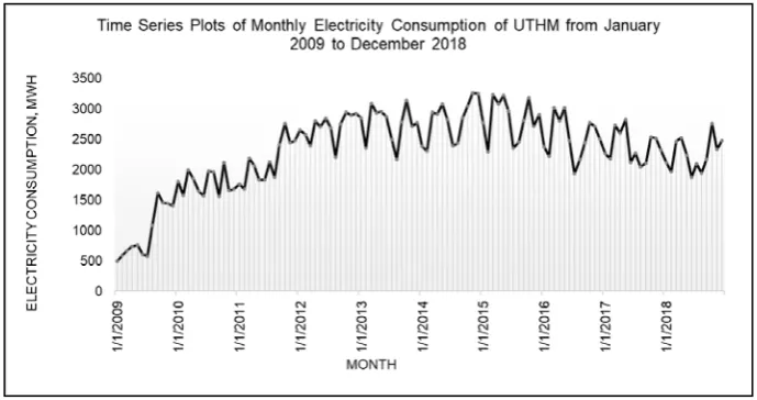
[image:3.595.125.470.373.555.2]

Figure 2 portrays the time series plots of monthly electricity consumption of UTHM from January 2009 to November 2018. The electricity consumption is range from around 500 MWh to 3500 MWh. The time series seems is not stationary and normal.

Figure 2. Time series plot without transformation

(4)

[image:4.595.124.470.77.654.2] [image:4.595.127.469.80.361.2]

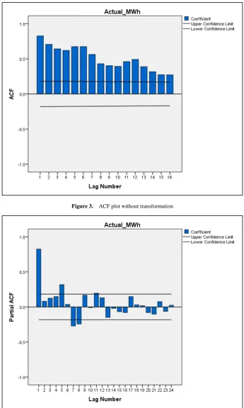
Figure 3. ACF plot without transformation

Figure 4. PACF plot without transformation

(5)

[image:5.595.81.513.75.318.2]

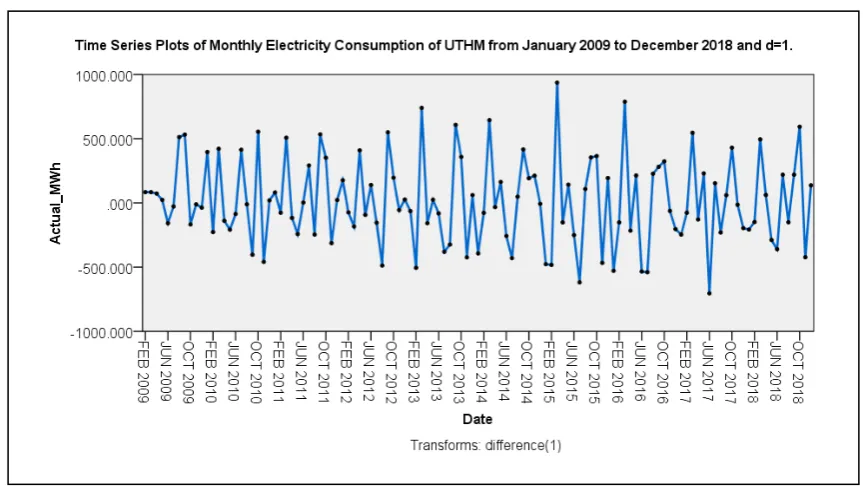
[image:5.595.124.470.376.653.2]

Figure 5. Time series plot with transformation d=1

Figure 5 shows a stationary and normal time series plot with a difference, d = 1. Hence, the ACF and PACF plots with transformation d = 1 were plotted as shown in Figure 6 and Figure 7.

(6)

[image:6.595.125.470.79.356.2]

Figure 7. PACF plot with transformation d = 1

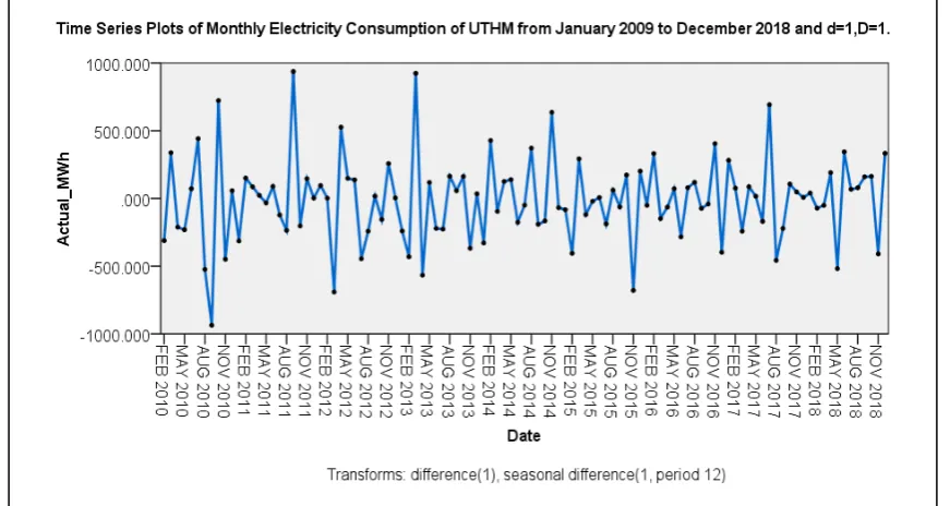
[image:6.595.81.517.442.674.2]

From figure 6, there is a significant autocorrelation at 12 lags (lag 12 and lag 24) which indicates that seasonality of data needed to be considered [21]. Hence first seasonal differencing needed to be done. The time series plot of monthly electricity consumption of UTHM from January 2009 to December 2018 with d = 1 and D = 1 was created as shown in Figure 8.

Figure 8. Time series plot with transformation d = 1 and D = 1

Figure 8 reveals a stationary and normal time series plot with seasonality proof after the transformation of difference, d

(7)

[image:7.595.126.470.80.357.2]

Figure 9. ACF plot with transformation d=1 and D=1

Figure 10. PACF plot with transformation d = 1 and D = 1

4.1.2. Model Identification

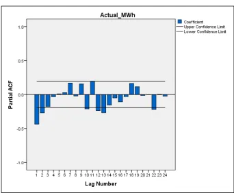
From the ACF plot in Figure 9, there is significant autocorrelation at Lags 1, 10 and 11 which will be the value of q. While the significant autocorrelation at Lag 12 indicates that the value of Q = 1.

From the PACF plot in Figure 10, there is significant

autocorrelation at Lags 1, 2 and 10 which will be the value of p. While the autocorrelation at Lag 12 presents but less significant, hence, it indicates that the value of P = 0 or P = 1.

[image:7.595.125.468.373.655.2]

(8)

needed to be considered in the models.

In this study, the lags 10 and 11 on the order AR and MA were ignored. That is because when building a model using the 10th-order lag and 11th-order lag, they produce a model that is not simple. [18].

There were 6 initial models being identified. The Identified SARIMA models were listed as followss: 1) SARIMA (1,1,1)(0,1,1)12

2) SARIMA (1,1,1)(1,1,1)12 3) SARIMA (2,1,1)(0,1,1)12 4) SARIMA (2,1,1)(1,1,1)12 5) SARIMA (0,1,1)(0,1,1)12 6) SARIMA (0,1,1)(1,1,1)12 4.1.3. Parameters Estimation

Table 1 displays parameter estimator (column 3) and the significance test (column 4). Column 4 indicates the significance of α value. The following hypothesis will be used to identify significant models:

H0: α > 0.05: Model insignificant

H1: α < 0.05: Model significant

4.1.4. Diagnosis

From Table 1, it is clearly shown that only SARIMA (0, 1, 1)(0, 1, 1)12 has met the assumptions of the model diagnostics.

[image:8.595.305.537.92.432.2]

The residual plots of ACF and PACF in Figure 11 shows the model is adequate as it shows a random variation from the origin zero (0), the points below and above are all uneven, hence the model fitted is adequate.

Table 1. Significant parameters of identified models

Model P Est. Sig. Result

SARIMA (1,1,1) (0,1,1)12

AR (1) 0.064 0.712 Several parameters

are insignificant. MA (1) 0.670 0.000*

SMA (12) 0.532 0.000*

SARIMA (1,1,1) (1,1,1)12

AR (1) 0.028 0.869

Several parameters

are insignificant. MA (1) 0.662 0.000*

SAR (12) -0.271 0.230

SMA (12) 0.243 0.326

SARIMA (2,1,1) (0,1,1)12

AR (1) -0.045 0.832

Several parameters

are insignificant. AR (2) -0.154 0.272

MA (1) 0.555 0.005*

SMA (12) 0.539 0.000*

SARIMA (2,1,1) (1,1,1)12

AR (1) -0.102 0.625

Several parameters

are insignificant. AR (2) -0.178 0.209

MA (1) 0.531 0.007*

SAR (12) -0.317 0.143

SMA (12) 0.212 0.377

SARIMA (0,1,1) (0,1,1)12

MA (1) 0.634 0.000* All

parameters are significant. ( Reject H0) SMA (12) 0.515 0.000*

SARIMA (0,1,1) (1,1,1)12

MA (1) 0.647 0.000* Several parameters

are insignificant. SAR (12) -0.287 0.194

SMA (12) 0.221 0.345

[image:8.595.126.470.460.731.2]

(9)

4.1.5. Forecast

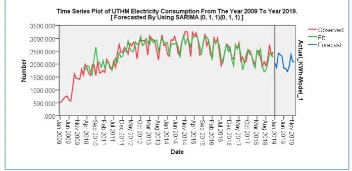
The forecasted plot of SARIMA (0, 1, 1)(0, 1, 1)12 through Box-Jenkin method is shown in Figure 12 and the forecasted results of the year 2019 were tabulated in Table 2.

[image:9.595.122.471.129.299.2]

Figure 12. Forecasted time series plot of UTHM electricity consumption from the year 2009 to 2019

Table 2. Result comparison for both methods.

Parameter Estimator Box-Jenkins Method Expert Modeler

Model SARIMA

(0, 1, 1)(0, 1, 1)12

SARIMA (0, 1, 1)(0, 1, 1) 12

MA(1) Est. = 0.634

Sig. = 0.000

Est. = 0.589 Sig. = 0.000

SMA (12) Est. = 0.515

Sig. = 0.000

Est.= 0.456 Sig.= 0.000

Model Statistics Box-Jenkins Method Expert Modeler Method SPSS

Stationary R-squared 0.365 0.349

R- squared 0.674 0.666

RMSE 254.400 255.098

MAPE 8.403 8.467

MaxAPE 70.212 71.204

MAE 191.254 192.102

MaxAE 1095.624 1111.109

Normalized BIC 11.253 11.171

Overall Significant 0.012 0.016

Forecasted Result Box-Jenkins Method, KWh Expert Modeler Method SPSS, KWh

Jan 2019 2044.922 2108.894

Feb 2019 1869.671 1959.184

Mar 2019 2426.835 2525.423

April 2019 2366.109 2493.836

May 2019 2303.708 2428.356

June 2019 1838.178 1977.722

July 2019 1833.007 2028.093

Aug 2019 1709.822 1915.090

Sept 2019 1903.277 2119.614

Oct 2019 2362.180 2614.828

Nov 2019 2091.124 2349.226

[image:9.595.72.524.340.758.2]

(10)

The forecasted part was enlarged for a clearer view as displayed in Figure 13.

Figure 13. An enlarged forecasted plot with data label

4.2. Expert Modeler

The forecasted plot, enlarged forecasted plot and residual plots of ACF and PACF from Expert Modeler SPSS are shown in Figure 14, Figure 15 and Figure 16 respectively.

Figure 14. Forecasted time series plot generated from Expert Modeler in SPSS

[image:10.595.123.470.95.268.2] [image:10.595.128.469.359.519.2] [image:10.595.126.471.472.727.2]

(11)

Figure 16. Residual ACF and PACF plots by Expert Modeler SPSS

4.3. Comparison of Box-Jenkins Method with Expert Modeler SPSS

The comparison of both Box-Jenkins method and Expert Modeler SPSS included Parameter Estimator, Model Statistics, and forecasted result as shown in Table 2. It reveals results generated from the Box-Jenkins method and Expert Modeler are approximately the same.

5. Conclusions

From the result obtained, it can be concluded that the Box-Jenkins method and Expert Modeler in SPSS are eligible to forecast the UTHM electricity consumption for the year 2019. However, Expert Modeler will be more advanced as compared to Box-Jenkins method which needs to manually examine the most suitable model from numerous models identified with various testing while Expert Modeler can finish the forecast in just several clicks.

In this paper, the electricity consumption of UTHM of the year 2019 can be forecasted by using SARIMA method in SPSS through Box-Jenkins method and Expert Modeler with the real data taken from January year 2009 to December year 2018. The SARIMA model to forecast the UTHM electricity consumption is SARIMA (0, 1, 1) (0, 1, 1)12. The Mean absolute percentage error (MAPE) of the forecasted result is 8.4%.

Acknowledgements

We wish to thank Mr. Shukur Saleh and Mr. Abd Rashid Puteh from Development and Maintenance Office, UTHM for providing us wth UTHM electricity consumption data, Dr. Maria Elena Nor for valuable suggestion of using SARIMA model, UTHM Tier 1 2018 research grant vote H258 and Fundamental Research Grant Scheme (FRGS) vote 1581 granted by Ministry of Education (MOE) Malaysia for financial support of this project.

REFERENCES

[1] S. Makridakis and R. J. Hyndman, Forecasting: Methods and Application. Journal of Statistical Assocoation, Vol.94, No.445, 345-346, 1984

[2] V. Lepojević & M.Anđelković-Pešić, Forecasting Electricity Consumption by Using Holt-Winters and Seasonal Regression Models. Series: Economics and Organization, Vol. 8, No.4, 424-431, 2011.

[3] Y. W. Lee, K. G. Tay & Y. Y. Choy, Forecasting Electricity Consumption Using Time Series Model. International Journal of Engineering and Technology, Vol. 7, No. 4.30, 218-223, 2018.

[image:11.595.127.468.79.355.2]

(12)

[5] K. G. Tay, Y. Y. Choy, & A. Huong, Forecasting Electricity Consumption Using Multiple Linear Regression. International Journal of Engineering and Technology, Vol. 7, No.4, 3515-3520, 2018.

[6] K. Panklib, C. Prakasvudhisam & D. Khummonqkol, Electricity Consumption Forecasting in Thailand Using an Artificial Neural Network and Multiple Linear Regression. Vol. 10, No.4, 427-434. 2015.

[7] P. K. Jain, W. Quamer, & R. Rajendra Pamula, Electricity Consumption Forecasting Using Time Series Analysis. International Conference on Advances in Computing and Data Sciences, 327-335. 2018.

[8] A.H. Erol, N. Özçelikkan, A. Tokgöz, S. Özel, S. Zaim, & O. F. Demirey, Time Series Methods and Neural Network, 118-127, 2012.

[9] G. Ogcu, O.F Demirey & S. Zaim, Forecasting Electricity Consumption with Neural Networks and Support Vector Regression. Procedia - Social and Behavioral Sciences, Vol. 58, 1576 – 1585, 2012.

[10] A. Bâra, and S. V. Oprea, Electricity Consumption and Generation Forecasting with Artificial Neural Networks, Advanced Applications Artificial Neural Networks, 119-139, 2017.

[11] K. Kandananond, Forecasting Electricity Demand in Thailand with an Artificial Neural Network Approach. Energies. Vol. 4, 1246-1257, 2011.

[12] K. P. Amber, R. Ahmad, M. W. Aslam, A. Kousar, M. Usman & M. S. Khan, Intelligent techniques for forecasting electricity consumption of buildings, Vol. 157, No.15, 886-893, 2018.

[13] F. Kaytez, M. C. Taplamacioglu, E. Cam & F. Hardalac, Forecasting electricity consumption: A comparison of regression analysis, neural networks and least squares support vector machines, Electrical Power and Energy Systems, Vol. 67, 431-438, 2015.

[14] M. A. Nokar, F. Tashtarian, & M. H. Y. Moghaddam, Residential power consumption forecasting in the smart grid using ANFIS system, 7th Int. Conf. On Computer and Knowledge Engineering, 1-9, 2017.

[15] M. Mordjaoui, and B. Boudjema, Forecasting and Modelling Electricity Demand Using Anfis Predictor, Journal of Mathematics and Statistics, Vol. 7, No. 4, 275-281, 2011.

[16] S. Barak, & S. S. Sadegh, Forecasting energy consumption using ensemble ARIMA–ANFIS hybrid algorithm, International Journal of Electrical Power and Energies, Vol. 82, 92-104, 2016.

[17] E. Z. Martinez, E. A. S. da Silva, & A. L. D. Fabbro, A SARIMA forecasting model to predict the number of cases of dengue in Campinas, State of São Paulo, Brazil, Rev. Soc. Bras. Med. Trop., Vol. 44, No.4, 436–40, 2011.

[18] A. Rusyana, Nurhasanaj, Marzuki and M. Flancia, Sarima Model for Forecasting Foreign Tourist at the Kualanamu International Airport, 12th International Conference on Mathematics, Statistics and Their Applications, 153-158, 2016.

[19] G. E. P. Box & G. Jenkins, Time Series Analysis: Forecasting and control, Holden-Day, San Francisco, CA, 1970.

[20] IBM SPSS Forecasting 20, 2011.